The way to Mannequin a Magnet Falling By means of a Solenoid
[ad_1]
Introduction
Modeling a magnet realistically is a job finest accomplished numerically. Even the simplified mannequin of two separated disks with uniform floor magnetization ##pm~sigma_M## entails elliptic integrals simplifying assumptions. As a mannequin, the purpose dipole could also be unrealistic to some however the math is tractable and accessible. The usefulness of the purpose dipole mannequin in electrodynamics is analogous to that of the purpose mass in kinematics and dynamics. It brings forth the salient options and serves as a place to begin for extra concerned remedies. Certainly, analyses of the falling magnet discovered within the literature depend on modifications of the purpose dipole equations with an eye fixed towards bringing their predictions into higher settlement with experiments.
The aim of this text is to collect in a single place what will be mentioned a few magnet dipole falling via a solenoid. A second article, now in preparation, has the identical aim however for a degree magnetic dipole falling via a strong conducting pipe.
The motional emf
The inverse Lorentz transformation equations for the parts of the electrical and magnetic fields are $$start{align}& mathbf{E}_{parallel}=mathbf{E’}_{parallel}~;~~mathbf{B}_{parallel}=mathbf{B’}_{parallel}nonumber & mathbf{E}_{perp} =gammaleft(mathbf{E’}_{perp} -mathbf{v}timesmathbf{B’}proper)~;~~mathbf{B}_{perp}=gammaleft(mathbf{B’}_{perp}-frac{1}{c^2}mathbf{v}timesmathbf{E’}proper).nonumber finish{align}$$
Take into account a magnetic level dipole ##mathbf{m}=m~hat z## falling with velocity ##mathbf{v}=v~hat z##. Taking “down” as constructive and for strange magnet velocities (##gamma approx 1##), we write in cylindrical coordinates,$$mathbf{E}_{perp}=-mathbf{v}occasions mathbf{B’}=-mathbf{v}occasions mathbf{B}=-v~hat ztimesleft(B_{rho}~hat {rho}+B_z~hat {z}proper)=-vB_{rho}~hat {theta}.$$The road integral ##int_a^b mathbf{E}_{perp}cdot dmathbf{l}## is the motional emf between factors ##a## and ##b##.
The relativistic therapy could be a bit an excessive amount of, but it surely helps get the indicators proper. Anyway, from right here on we’ll discontinue the usage of primes to indicate coordinates within the transferring body. As an alternative, we’ll use primes for supply coordinates and no primes for coordinates of factors of curiosity. Integrals will likely be taken over primed coordinates.
A single ring
At focal point ##mathbf{r}(rho ,z)## when the dipole is at ##mathbf{r’}(rho’,z’)## the dipolar discipline is $$mathbf{B}=frac{mu_0}{4pi} left[ frac{ left(3 mathbf{m}cdot (mathbf{r}-mathbf{r}’))(mathbf{r}-mathbf{r}’)-|mathbf{r}-mathbf{r}’|^2 mathbf{m}right)}{|mathbf{r}-mathbf{r}’|^5} -frac{mathbf{m}}{ |mathbf{r}-mathbf{r}’|^3} right].$$We place the dipole on the ##z##-axis and orient it in order that ##mathbf{m}=m~hat z##. At ##rho=a##, the radial element of the magnetic discipline is $$B_{rho}=frac{3mu_0ma}{4pi} frac{ z-z’} {left[a^2+(z-z’)^2right]^{5/2}}.$$
The motional emf in a coaxial single ring of radius ##a## at ##z’## is $$start{align}textual content{emf}_{textual content{ring}}=int mathbf{E}_{perp}cdot dmathbf{l}=-vB_{rho}(2pi a) = -frac{3mu_0ma^2}{2} frac{ (z-z’)~v} {left[a^2+(z-z’)^2right]^{5/2}}.finish{align}$$Notice that the ring may very well be an intangible loop, not essentially conducting, and the emf round it could nonetheless exist. If, nevertheless, the ring is a conducting loop, there will likely be an induced present in it. A plot of the spatial dependence of the emf is proven in Determine 1 beneath. We observe that when the dipole is farther than about 4 radii from the ring’s middle, the emf is beneath 1% of its peak worth.
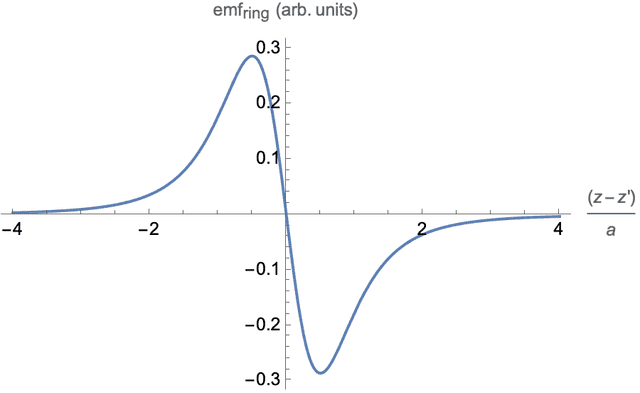
Determine 1. Single ring emf as a perform of dipole place.
Because the dipole falls in free area, a wave of motional emf with the waveform proven in Determine 1 is touring with velocity ##v(t)## down an intangible tube consisting of loops of radius ##a.## Within the subsequent part, we’ll discover what to anticipate when a conducting finite solenoid of radius ##a## occupies a part of that area.
From ring to solenoid
We think about the solenoid as a stack of ##N## turns. The start of the ##ok##th flip is the tip of the ##(k-1)##th and the tip of the ##ok##th flip is the start of the ##(ok+1)##th. Thus, the turns are a set of rings linked in collection. We’re looking for an expression for the emf throughout the free ends of a solenoid of ##N## turns, radius ##a##, and size ##L##. Will probably be an integral of ##textual content{emf}(z)## over the size of the solenoid.
The variety of rings in a stack of top ##dz’## is ##dn=dfrac{N}{L}dz’##. Integrating over the size, $$start{align}textual content{emf}(z)=frac{N}{L}int_{frac{-L}{2}}^{frac{L}{2}}textual content{emf}_{textual content{ring}}dz’=frac{mu _0 N m a^2}{2 L} left{ frac{v}{left[a^2+left(z-frac{L}{2}right)^2right]^{3/2}}-frac{v}{left[a^2+left(z+frac{L}{2}right)^2right]^{3/2}}proper}.finish{align}$$
We assume that the dipole has mass and is in free fall. If the solenoid ends are open, there will likely be an emf throughout them however no present. Even when a voltmeter is linked to measure the emf, the present via it’s anticipated to be negligible . In both case, eddy present braking is negligible and we’ll ignore it along with air resistance. Underneath these circumstances, the usual kinematic equations underneath fixed acceleration apply. Taking the origin on the midpoint of the solenoid, we write an expression for the place of the dipole. We assume that it begins from relaxation at top ##h## above the highest of the solenoid (##z_0=-h-frac{L}{2}##.) Substituting $$z=(-h-frac{L}{2}+frac{1}{2}g~t^2)~textual content{ and }~v=g~t$$ in equation (2), we acquire the emf throughout the solenoid as a perform of time. $$start{align}textual content{emf}(t)=frac{mu _0 N m a^2}{2 L} left{ frac{g~t}{left[a^2+left(-h-L+frac{1}{2}g~t^2right)^2right]^{3/2}}-frac{g~t}{left[a^2+left(-h+frac{1}{2}g~t^2right)^2right]^{3/2}}proper}finish{align}$$
The emf profile
Determine 2 beneath is a plot of emf(t) vs ##t## with out the general multiplicative fixed. For the plot, we used ##g=980## for the acceleration, ##a=1## for the radius, ##h=6a## for the discharge top above the highest and ##L=10 a## for the size. Thus, if the items for the radius ##a## are centimeters, the numbers on the abscissa will likely be seconds. The strong vertical grid strains mark the occasions when the dipole is on the prime, midpoint, and backside of the solenoid. The pairs of crimson dashed strains mark the occasions when the dipole is inside one solenoid diameter (##pm~2a##) from the highest (left) and the underside (proper).
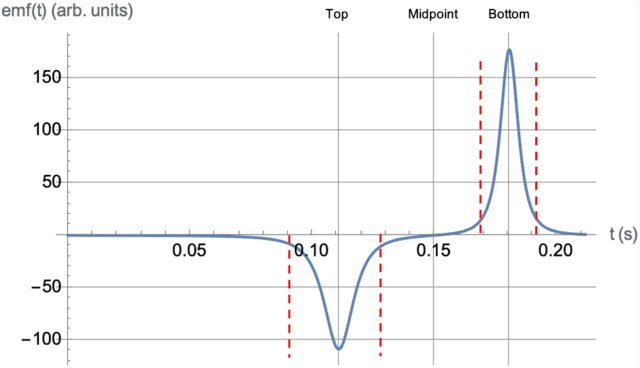
Determine 2. Solenoid emf as a perform of time.
Alternatively, we will acquire an expression for the emf as a perform of place ##z## by substituting ##v=sqrt{2g[z-(-h-frac{L}{2})]}## in equation (2) to get $$start{align}textual content{emf}(z)=frac{mu _0 N m a^2}{2 L} left{frac{sqrt{2 g left(z+h+frac{L}{2}proper)}}{left[a^2+left(z-frac{L}{2}right)^2right]^{3/2}}-frac{sqrt{2 g left(z+h+frac{L}{2}proper)}}{left[a^2+left(z+frac{L}{2}right)^2right]^{3/2}}proper}.finish{align}$$A plot of the emf(##z##) vs. ##z## just isn’t proven as a result of it’s an identical to the one in determine 2 apart from the labeling of the abscissa. Each plots characteristic extrema, one detrimental and one constructive, with a area between when/the place the emf is close to zero. That is qualitatively according to Faraday’s regulation. The magnetic flux modifications most quickly when the dipole is close to the ends and hardly in any respect when it’s close to the center of the solenoid.
Time period corrections
Examination of determine 2 reveals that the extrema happen when the dipole is close to the ends of the solenoid. At ##z=+L/2## the primary time period in equation (4) has a most whereas the second time period is small; the reverse is true at ##z=-L/2##. An actual willpower of the extrema would contain fixing ##frac{d}{dz}textual content{emf}(z)=0##, a frightening job. Contemplating, nevertheless, that the true extrema are very near ##z=pm frac{L}{2}##, it’s expedient to do collection expansions of equation (4) about ##z=pm frac{L}{2}## to second-order and discover corrections to the zeroth-order phrases. Right here, we summarize the outcomes and relegate among the particulars to the Appendix.
The fractional corrections to the place and worth of the minimal are $$frac{delta z}{(-L/2)}=-5.5times 10^{-3}~;~~frac{delta(textual content{emf})}{textual content{emf}(-L/2)}=1.1times 10^{-3}.$$The corresponding numbers for the utmost are $$frac{delta z}{(+L/2)}=2.1times 10^{-3}~;~~frac{delta( textual content{emf})}{textual content{emf}(L/2)}=1.6times 10^{-4}.$$The numbers present that the corrections have a small impact on the zeroth order phrases. Thus, we’ll ignore them and make the algebra simpler.
A relation between amplitudes
We outline as amplitudes the magnitudes of the extrema of ##textual content{emf}(t)## (Determine 2). Within the approximation that the extrema happen at ##z=pm ~frac{1}{2}##, equation (4) provides, the amplitudes $$start{align} & A_1=left|textual content{emf}(-L/2)proper|=sqrt{2 g h}left[frac{1}{a^3}-frac{1}{left(a^2+L^2right)^{3/2}}right]nonumber & A_2=textual content{emf}(+L/2)|=sqrt{2 g (h+L)}left[frac{1}{a^3}-frac{1}{left(a^2+L^2right)^{3/2}}right].nonumber finish{align}$$
We write the distinction between the 2 equations as $$start{align} & A_2-A_1=textual content{const.} left(sqrt{frac{2 (h+L)}{g}}-sqrt{frac{2 h}{g}}proper) nonumber & textual content{the place }textual content{const.}=frac{mu _0 N m a^2}{2 g L}left[frac{1}{a^3}-frac{1}{left(a^2+L^2right)^{3/2}}right].nonumber finish{align}$$We acknowledge the expression in parentheses multiplying the fixed because the transit time ##T## of the dipole from one finish of the solenoid to the opposite. This simplifies the equation much more to $$start{align}A_2-A_1=(textual content{const.})occasions T.finish{align}$$
It’s simple to think about an experimental protocol to check equation (5) with tools that samples and data the emf throughout the solenoid as a perform of time. Nevertheless, one ought to make sure that beginning heights ##h## are larger than the efficient dipole vary of 4 solenoid radii. This can decrease experimental uncertainties that change into vital at small values of ##h##. A PF thread posted by @billy_t right here describes such an experiment. Nevertheless, the evaluation centered on the amplitudes themselves and never on their relation to the time of transit.
Abstract
Modeling a magnet as a degree dipole falling via a solenoid is ample to supply a wise description of the form and basic options of the emf(##t##) curve that’s in settlement with what one would count on qualitatively. The flux varies most quickly when the dipole is coming into and exiting the solenoid and least quickly when it’s close to the solenoid’s center. The amplitude of the correct peak is larger than the left. This occurs as a result of its width is narrower for the reason that dipole is transferring quicker, but the realm underneath the curve is identical. It’s unlikely {that a} extra practical mannequin of the magnet will lead to a special interpretation of those options. A complicated mannequin wants subtle information evaluation to match it, maybe one involving a point-by-point simulation of your entire curve.
Acknowledgments
I thank @billyT_ for posting the thread quoted above; it seeded this perception. Additionally, the participation of @haruspex and @Charles Hyperlink honed my pondering and is significantly appreciated.
Appendix
The work proven right here was Mathematica-assisted. In equation (4) we first drop ##g## and substitute decreased lengths ##lambda=L/a,~eta=h/a##. Then increase the equation for small values of ##epsilon = zpm lambda/2## to second order. Every growth yielded a quadratic expression ##Aepsilon^2+Bepsilon+C.## Setting the spinoff equal to zero and fixing for ##epsilon## provides ##epsilon=frac{-B}{2A}##. Omitting the gory particulars, the corrections for the minimal on the left and the utmost on the correct are:
$$start{align} & epsilon_{textual content{min}} =frac{2 eta left(lambda ^2+1right) left[left(lambda ^2+1right)^{5/2}-left(6 eta lambda +lambda ^2+1right)right]}{left(12 eta ^2+1right) left(lambda ^2+1right)^{7/2}+12 eta ^2 left(4 lambda ^2-1right)+12 eta lambda left(lambda ^2+1right)-left(lambda ^2+1right)^2}nonumber & epsilon_{textual content{max}} =frac{ 2 left(lambda ^2+1right) (eta +lambda ) left[6 eta lambda +left(lambda ^2+1right)^{5/2}+5 lambda ^2-1right]} {12 eta ^2 left(4 lambda ^2-1right)+12 eta lambdaleft(7 lambda ^2-3right) +left(lambda ^2+1right) left[12 left(lambda ^2+1right)^{5/2} (eta +lambda )^2+1right]+left(35 lambda ^4-26 lambda ^2-1right)}nonumber finish{align}$$Determine 3 exhibits a element of determine 2 within the neighborhood of the utmost. The vertical line is on the corrected worth of ##z/a##. The zeroth order time period of the growth is to its left at ##z/a=5.00##.
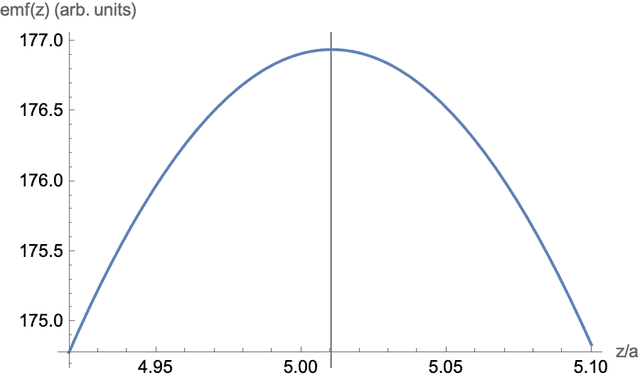
Determine 3. Element of the correction to the zeroth order time period.
[ad_2]