All Quantity Methods That We Have
[ad_1]
A whole ebook may simply be written concerning the historical past of numbers from historical Babylon and India, over Abu Dscha’far Muhammad ibn Musa al-Chwarizmi (##sim ## 780 – 845), Gerbert of Aurillac aka pope Silvester II. (##sim ## 950 – 1003), Leonardo da Pisa Fibonacci (##sim## 1170 – 1240), Johann Carl Friedrich Gauß (1777 – 1855), Sir William Rowan Hamilton (1805 – 1865), to Kurt Hensel (1861 – 1941). This may lead too far. As a substitute, I need to take into account the numbers by their mathematical that means. However, I’ll attempt to describe the arithmetic behind our quantity methods as merely as potential.
I like to think about the discovering of zero as the start of arithmetic: Somebody determined to depend what wasn’t there! Simply sensible! Nevertheless, the reality is as typically much less glamorous. Babylonian accountants wanted a placeholder for an empty area for the quantity system they used of their books. The digits zero to 9 have been first launched in India. In Sanskrit, zero stands for vacancy, or nothingness.
From Zero To Rational Numbers
It began with counting, the pure numbers ##1,2,3,ldots## John von Neumann proposed the next set-theoretical definition
$$
start{array}{lll}
0&={}&=emptyset
1&=0’={0}&={emptyset}
2&=1’={0,1}&={emptyset,{emptyset}}
&;vdots &;vdots
n+1&=n’={0,1,2,ldots,n}&=ncup {n}
finish{array}
$$
That is already arithmetic and never pure anymore. It incorporates the idea of zero as its start line, not one, it implicitly makes use of the idea of cardinality, and most of all, the idea of a successor, famous by a main. The successor is what finally defines a pure quantity. Its existence is commonly known as the Peano axiom, though Giuseppe Peano (1858 – 1932) initially listed 5 axioms to outline the pure numbers. Nevertheless, it’s the necessary one:
Each pure quantity has a (new) successor.
That is pure since we will all the time have yet one more. Nevertheless, it isn’t self-evident. If we outline ##0=textual content{[ OFF ]}## and ##1=textual content{[ ON ]}##, the 2 states of a mild swap, then the successor of 1 is the predecessor of the opposite. We’re caught with ##{0,1}## and don’t get a brand new successor. The successor axiom can’t be overestimated. For instance, it additionally defines an ordering, the successor is greater than the predecessor. This won’t work for the sunshine swap! The successor axiom guidelines our every day life, the sunshine switches in our digital units, particularly our computer systems.
One other consequence of the successor axiom is the existence of a predecessor for all numbers apart from the primary one. Whether or not the primary one is ##1## or ##0## can’t lastly be determined. Personally, I take into account the zero, a quantity that counts what isn’t there, an achievement of mankind. I, due to this fact, don’t take into account zero as a pure quantity and begin with one and distinguish between
start{align*}
mathbb{N}={1,2,3,ldots};textual content{ and };mathbb{N}_0={0,1,2,3,ldots}.
finish{align*}
Now that folks may depend, in addition they may examine sizes. The query for an answer to
$$
a+x=b
$$
was a matter of time. It really works fantastic so long as ##a<b,## however what if ##a>b##? We may resolve ##b+x=a## as a substitute, however isn’t this a step too many? Leopold Kronecker (1823 – 1891) is understood for his citation
Die ganzen Zahlen hat der liebe Gott gemacht. Alles andere ist Menschenwerk.
(God made the integers, all the remaining is the work of man.)
We may begin a philosophical debate at this level, and for instance point out that almost all mathematicians are Platonists who imagine that nothing is man-made, and all is already existent, ready to be discovered. Nevertheless, I’m afraid that already Kronecker’s view is extra poetic than lifelike. I imagine, that the integers had been made by accountants, or ought to I say discovered? As quickly as individuals had a ebook that famous harvest, earnings, and taxes, as quickly they wanted all integers. I desire the mathematical standpoint. The pure numbers construct a half-group in accordance with the binary operation addition. The sum of pure numbers is a pure quantity once more, and the order of addition doesn’t make a distinction: ##a+b=b+a## (commutative) and ##a+(b+c)=(a+b)+c## (associative). If we need to resolve ##a+x=b## in all circumstances, then we’d like a impartial aspect ##a+x=a## which we name ##x=0,## and inverses ##a+x=0## which we name destructive numbers ##x=-a##. Geared up with each we get the integers
$$
mathbb{Z}={ldots,-4,-3,-2,-1,0,1,2,3,4,ldots}
$$
that type a so-called group due to the existence of a impartial aspect, and inverse components. It’s a pure extension of pure numbers which led to Kronecker’s comment. Each, pure numbers and integers enable one other binary operation: multiplication that’s commutative and associative, too:
“Expensive Sultan, we count on 1000 occasions 10 bushels of wheat this 12 months.”
The 2 binary operations are associated by the distributive legislation
$$
acdot (b+c)=acdot b +acdot c
$$
You will need to observe that this legislation is the one connection between the 2 operations. It defines
$$
acdot 0=acdot (a+(-a))=acdot a +(acdot (-a))=a^2+(-a^2)=0
$$
Units with these two operations and the distributive legislation are known as rings. Multiplication doesn’t construct a gaggle, solely a half-group. It comes with an computerized impartial aspect, one, however we would not have multiplicative inverses. And even worse,
$$
acdot 0 = 0 = bcdot 0
$$
makes it unattainable to resolve the equation ##1=xcdot 0 =0.## Therefore, no matter we are going to do to outline multiplicative inverses, zero received’t be invited to the celebration. That is the rationale why division by zero is forbidden. It’s as a result of ##1neq 0.##
Rings for which a product can solely change into zero if one of many elements is already zero are known as integral domains. This isn’t all the time the case. For example
$$
start{bmatrix}0&1�&0end{bmatrix}cdotbegin{bmatrix}0&1�&0end{bmatrix}=start{bmatrix}0&0�&0end{bmatrix}
$$
Integral domains, nonetheless, enable the constructing of so-called quotient fields. A discipline is a hoop through which we have now multiplicative inverses for all components besides the zero, after all, i.e. through which we will divide. The development goes as follows. Let ##R## be the integral area and ##S=R-{0}## a multiplicative set. It’s a set that’s closed beneath multiplication, i.e. multiplication stays within the set. Subsequent, we outline an equivalence relation on ##Rtimes S## by
$$
(a,b) sim (c,d) Longleftrightarrow acdot d= bcdot c
$$
The set of all equivalence courses ##Q=Rtimes S/sim## is then the quotient discipline of the integral area ##R.## Utilized to the integers ##R=mathbb{Z}, ## and writing ##(a,b)=a/b## we get the sector of the rational numbers
$$
mathbb{Q}=left{left.dfrac{a}{b}, proper| ,ain mathbb{Z},bin mathbb{Z}-{0}proper}.
$$
The trick with the equivalence courses makes positive, that we would not have to differentiate between, say
$$
(1,2)=dfrac{1}{2}=dfrac{2}{4}=dfrac{-3}{-6}=ldots
$$
It’s crucial in case we need to take into account different integral domains, different multiplicative units, and therewith different quotient fields. For instance, there’s a quotient discipline for the ring of polynomials, the rational operate discipline, and the quotients of polynomials. By defining the rational numbers, we prolonged the multiplicative set ##mathbb{Z}-{0}## to a multiplicative group as a result of we will now divide, and thus resolve the equations
$$
acdot x=b.
$$
Prime Fields And Area Extensions
A primary discipline is the smallest discipline that’s included in one other. The sphere of rational numbers is the prime discipline of the actual numbers. It’s also the prime discipline of itself. There isn’t a smaller discipline included within the rationals. This isn’t a shock as a result of we solely added absolutely the minimal to assemble quotients of integers. However even the traditional Greeks who had been masters of geometry knew that the size of the diagonal in a sq. of facet size one is a quantity that isn’t rational, ##sqrt{2}##. They known as such numbers irrational, not rational. Their proof was simple. If ##sqrt{2}in mathbb{Q}## then we will write a main issue decomposition of ##2## as
$$
2=dfrac{a^2}{b^2} = p_1^{k_1}cdotldotscdot p_2^{k_r} in mathbb{Z}
$$
This may solely be if ##p_1=2,k_1=1.## All powers on the best, then again, are even since we have now a quotient of squares. Therefore our assumption was incorrect that ##sqrt{2}## is rational as a result of we can’t derive one thing false from one thing true. If we add ##sqrt{2}## to the rational numbers,
$$
mathbb{Q} subsetneq mathbb{Q}(sqrt{2})
$$
then we get a bigger discipline. Including right here means, that we add all polynomial expressions that contain ##sqrt{2}.## These aren’t many since ##sqrt{2}^2=2in mathbb{Q}.## With that we have now mechanically ##-sqrt{2}## and the one query is whether or not we have now the multiplicative inverse of ##sqrt{2},## too. Now,
$$
left(sqrt{2}proper)^{-1} = dfrac{1}{sqrt{2}}=dfrac{sqrt{2}}{sqrt{2}^2}=dfrac{sqrt{2}}{2}in mathbb{Q}(sqrt{2})
$$
is once more a polynomial expression with rational numbers and ##sqrt{2}.## Comparable could be completed with the diagonal of the dice, ##sqrt{3},## or on the whole every other quantity that’s the zero of a polynomial just like the diagonal of the sq. ##x^2-2=0## or of the dice ##x^2-3=0## are. These numbers are known as algebraic over ##mathbb{Q}## since they resolve a polynomial, an algebraic equation
$$
alpha^n+c_1alpha^{n-1}+c_2alpha^{n-2}+ldots+c_{n-1}alpha +c_0 =0
$$
These discipline extensions are constructed by including zeros of polynomials
$$
mathbb{Q} subseteq mathbb{Q}(alpha )subseteq mathbb{Q}(alpha ,beta )subseteq mathbb{Q}(alpha ,beta ,gamma )subseteq ldots
$$
are additionally known as algebraic. We all know since 1761 or 1767 from Johann Heinrich Lambert (1728 – 1777) that ##pinotin mathbb{Q}.## Since 1882 we all know from Carl Louis Ferdinand Lindemann (1852 – 1939) that ##pi## isn’t even algebraic over ##mathbb{Q}.## Which means that there is no such thing as a polynomial with rational coefficients that has ##pi## as a zero. However, we will construct ##mathbb{Q}(pi)## by permitting all integer powers of ##pi## in rational expressions. What we get then is a so-called transcendental extension of the rationals that’s the identical because the rational operate discipline in a single variable
$$
mathbb{Q}(pi) cong mathbb{Q}(x) =left{left.dfrac{p(x)}{q(x)}, proper| ,p(x)in mathbb{Q}[x], , ,q(x)in mathbb{Q}[x]-{0}proper}.
$$
Even when we constructed many, even countable infinitely many algebraic and transcendental discipline extensions of the rational numbers, even then we’d by no means get to the sector of the actual numbers. This can’t be dealt with by including some zeros of polynomials and a few transcendental numbers like ##pi, e## or ##2^{sqrt{2}}## alone. This may take a brand new methodology.
Topological Completion
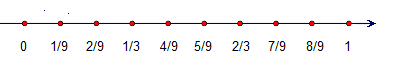
If we draw a quantity line and mark rational numbers then two issues catch the attention:
- irrespective of how shut we glance, there’ll all the time be infinitely many rational numbers between any two chosen rational ones
- irrespective of how shut we glance, there’ll all the time be infinitely many irrational numbers between any two chosen rational ones
The rational numbers have gaps, the quantity line doesn’t. The query is thus: how will we fill the gaps between ##mathbb{Q}## and ##mathbb{R}##? One methodology to attain this aim was offered by Julius Wilhelm Richard Dedekind (1831 – 1916) by way of so-called Dedekind cuts which are primarily based on the remark, that we will exactly find any hole between rational numbers by telling which rational numbers are to the left of it and that are to the best of it. This methodology principally follows the instinct of the geometrical view of the quantity line. One other methodology that’s the popular one these days was offered by up to date Georg Ferdinand Ludwig Philipp Cantor (1845 – 1918). This methodology is analytical. It doesn’t have a look at what’s outdoors a niche, it describes what’s in a niche, i.e. the place we find yourself after we take into account endlessly nested intervals. E.g.
$$
sqrt{2}=1.414213562373095048801688724209 ldots
$$
which implies it’s between
start{align*}
1&textual content{ and } 2
1.4=dfrac{14}{10}&textual content{ and } 1.5=dfrac{15}{10}
1.41=dfrac{141}{100}&textual content{ and } 1.42=dfrac{142}{100}
1.414=dfrac{1414}{1000}&textual content{ and } 1.415=dfrac{1415}{1000}
1.4142=dfrac{14142}{10000}&textual content{ and } 1.4143=dfrac{14143}{10000}
&;ldots
finish{align*}
These intervals change into shorter and shorter. And there is just one quantity, ##sqrt{2},## that’s contained in all intervals. We write
$$
sqrt{2}in left[dfrac{a_n}{10^n},dfrac{b_n}{10^n}right] textual content{ for all }nin mathbb{N} Longrightarrow lim_{n to infty}dfrac{a_n}{10^n}=lim_{n to infty}dfrac{b_n}{10^n}=sqrt{2}
$$
which implies that ##sqrt{2}## is the restrict of the interval borders. The borders get narrower and narrower, and so do the distances between ##a_n/10^n## and ##a_{n+1}/10^{n+1}## and likewise between ##b_n/10^n## and ##b_{n+1}/10^{n+1}.## Sequences with this property are known as Cauchy sequences, named after Augustin-Louis Cauchy (1789 – 1857). So all we have now to do to get all actual numbers (as much as some technical particulars) is so as to add all limits of rational Cauchy sequences
$$
mathbb{R}=left{left.r, proper| ,textual content{ there’s a Cauchy sequence }(C_n)_{nin mathbb{N}}subseteq mathbb{Q}textual content{ such that }lim_{n to infty}C_n=rright}.
$$
It’s known as the topological completion of the rational numbers because it fills all of the gaps on the quantity line that aren’t rational numbers. We assemble the actual numbers in a means that ensures the existence of these limits.
Notice that we didn’t outline the actual numbers by their decimal illustration! ##sqrt{2}=1,414213562373095048801688724209 ldots## shouldn’t be an actual quantity since we can’t write it all the way down to the top. It’s going to all the time be a rational quantity. The dots point out that it goes on eternally. It’s the restrict that’s hidden within the dots. E.g.
$$
0.999999ldots =0.overline{9}=sum_{ok=1}^infty dfrac{9}{10^ok}=lim_{n to infty} underbrace{sum_{ok=1}^n dfrac{9}{10^ok}}_{=a_n}=dfrac{1}{1-(9/10)}-9=1
$$
The decimal illustration is just a software that permits us to speak. The actual quantity it represents is the restrict. The totally different illustration of 1 by ##0.999999ldots ## on one hand and ##1## on the opposite is what I meant by technical particulars. It implies that mathematical rigor requires some further arguments to match the 2 representations.
Algebraic Closure
We started our journey by fixing the equations ##a+x=b## and ##acdot x=b.## Then we used geometrical strategies to outline the quantity line. But, there are nonetheless equations we can’t resolve:
$$
x^2+1=0.
$$
This polynomial equation has no rational or actual options. Nevertheless, we already know what must be completed so as to add zeros of polynomials
$$
mathbb{Q}subseteq mathbb{R}subseteq mathbb{R}( i )
$$
the place ##i## solves ##x^2+1=0.## Much like the process we used for ##sqrt{2},## we now get the advanced numbers
$$
mathbb{C}= mathbb{R}(i)=mathbb{R} + icdot mathbb{R}.
$$
It was roughly already recognized to the Babylonians that
$$
x^2+px+q=0 textual content{ implies } x= dfrac{1}{2}left(-ppm sqrt{p^2-4q}proper)
$$
and that the foundation can’t be solved in any case. The essential level by naming ##sqrt{-1}= i ## is that we will calculate with it with out even understanding what it’s, just by respecting ##i^2 =-1.##
It’s a non-real answer, an imaginary quantity. However what makes ## i ## so particular compared to all different algebraic numbers we already captured on the actual quantity line? Sure, it isn’t on the road, so we discovered an instance of a lacking algebraic quantity. Are there extra of them that we have now to take into accounts? The reply to this query is no, and that is what makes ## i ## so particular.
Each advanced polynomial has a fancy zero.
This theorem is so necessary that it’s known as the elemental theorem of algebra. However what makes it elementary? It’s the lengthy division that makes it. Say we have now a fancy polynomial ##p_0(x)in mathbb{C}[x]## and a fancy zero ##p_0(a_0+ib_0)=0.## Then we will write
$$
p_0(x)=p_1(x)cdot (x-(a_0+ib_0)) textual content{ with } deg p_1(x) < deg p_0(x)
$$
We now proceed by the subsequent zero, a zero of ##p_1(x),## and cut back the diploma once more and proceed till we find yourself with a linear polynomial and
$$
p_0(x)=(x-(a_0+ib_0))cdot(x-(a_1+ib_1))cdotldotscdot (x-(a_n+ib_n))
$$
By merely including the imaginary unit ##i,## we’re capable of resolve all advanced polynomial equations, i.e. there are not any algebraic numbers left so as to add. The advanced numbers are algebraically closed.
Quaternions and Octonions
The advanced numbers could be visualized as factors within the advanced aircraft as a result of ##mathbb{C}=mathbb{R}+icdotmathbb{R},## and Sir William Rowan Hamilton (1805 – 1865) spent years determining an analogous building for the three-dimensional area. He failed. However at the very least he discovered a four-dimensional building
$$
mathbb{H}=mathbb{R}+icdotmathbb{R}+j cdotmathbb{R}+kcdotmathbb{R}
$$
which we now name Hamilton numbers or quaternions. Sadly, he had to surrender commutativity. The multiplication desk is given by
$$
start{array}c
hline cdot &;,1;, &i&j&ok
hline ;1;&1&i&j&ok
hline i&i&-1&ok&-j
hline j&j&-k&-1&i
hline ok&ok&j&-i&-1
hline
finish{array}
$$
which isn’t symmetric. Such a skew discipline is named a division algebra. Ferdinand Georg Frobenius (1849 – 1917) proved in 1877 that there are solely these three associative, finite-dimensional, actual division algebras, ##mathbb{R},mathbb{C},mathbb{H}.##
Why will we emphasize associativity? It’s as a result of there may be one other finite-dimensional, actual division algebra if we drop the necessities of a commutative and an associative multiplication, the Cayley numbers or octonions. They’ve eight dimensions over the actual numbers and are a non-associative extension of the quaternions. Octonions had been first described by John Thomas Graves (1806 – 1870) in a letter to Sir William Rowan Hamilton in 1843. They had been independently found and first printed by Arthur Cayley (1821 – 1895) in 1845,
$$
mathbb{O}=mathbb{R}+icdot mathbb{R}+jcdot mathbb{R}+kcdot mathbb{R}+lcdot mathbb{R} +mcdot mathbb{R}+ncdotmathbb{R}+ocdot mathbb{R}.
$$
Attribute
The octonions are principally the top of this line. They symbolize the borderline between fields of attribute zero and buildings known as algebras. The road isn’t fairly sharp because the notation of division algebras suggests. Algebras are rings which are additionally vector areas and there are a lot of of them, e.g. Boolean, genetic, Clifford, Jordan, Graßmann, Lie, or – for string principle physicists – Virasoro algebras, and so on. Wait! What does attribute imply? We’ve used ##1neq 0## to this point which is smart since in any other case, each calculation would lead to zero. However what occurs if set
$$
underbrace{1+1+1+ldots+1+1}_{ntext{ occasions}}=0,
$$
which isn’t as far-fetched because it sounds since ##1+1=0## inside our discipline of sunshine swap states ##{0,1}.##
One other instance could be the twelve-hour mark on the face of a clock. If we take into account ##1## as ##+1## hour, then ##1+1+1+1+1+1+1+1+1+1+1+1=0.## Nevertheless, we have now
$$
3cdot 4 = 0text{ and }2cdot 6 = 0
$$
in that case which doesn’t enable us a division by ##2,3,4## or ##6,## if we nonetheless need ##1neq 0.## However, if we have now a main ##p##
$$
underbrace{1+1+1+ldots+1+1}_{ptext{ occasions}}=p=0,
$$
then we received’t get into that hassle. Such a set would encompass ##p## many components and actually, represents a discipline through which we will carry out all 4 fundamental operations,
$$
mathbb{F}_p={0,1,2,ldots,p-1}.
$$
We name ##p## the attribute of ##mathbb{F}_p.## In case ##p=infty ,## i.e. sums of ones won’t ever be zero as in our regular fields ##mathbb{Q},mathbb{R},mathbb{C},## we are saying that the attribute of such fields is zero. It is a conference as a result of mathematicians don’t like to think about infinity as a quantity. Nevertheless, they don’t have any drawback calling traits ##p## finite with a view to distinguish them from ##0.## All fields ##mathbb{F}_p## are prime fields as a result of they solely encompass the minimal of crucial components, and the sunshine swap is
$$
mathbb{F}_2={[text{ ON }],[text{ OFF }]}={0,1}.
$$
A discipline of attribute ##p=2## has no indicators
$$
1+1=0 textual content{ implies } 1=-1.
$$
That is particularly necessary in all circumstances the place indicators play a vital function; e.g. for Graßmann or Lie algebras!
Algebraic and transcendental extensions could be constructed simply as within the case of the rational numbers. However the identification ##p=0## has a humorous consequence
$$
(x+y)^p=sum_{j=0}^p binom{p}{j} x^{p-j}y^j=x^p+pcdot x^{p-1}y+ldots+pcdot xy^{p-1}+y^p=x^p+y^p.
$$
p-adic Numbers
Absolutely the worth of a quantity on the quantity line measures its distance from zero. It’s known as a valuation, an Archimedean valuation to be actual. Which means that we will all the time put the smaller size collectively so many occasions that it exceeds the bigger size.
$$
|N cdot a|>|b|>|a|>0quad (Nin mathbb{N})
$$
Kurt Hensel (1861 – 1941) offered in 1897 a discipline extension of the rational numbers for which this isn’t true any longer. We’re, regardless of the title of this part, again within the attribute ##0## case once more because the rational numbers shall be our prime discipline. Say we have now a main ##p## and ##a=p^r cdot m’; , ;b = p^s cdot n’.## Then
$$
left|dfrac{a}{b}proper|_p = start{circumstances} p^{-r+s} &textual content{ if } a neq 0 0&textual content{ if }a=0end{circumstances}
$$
defines a valuation that’s not Archimedean. However, it nonetheless defines a distance by
$$
d(a,b)=|a-b|_p.
$$
With the space comes the chance of a topological completion, the ##p##-adic numbers
$$
mathbb{Q}_p=left{left.dfrac{a}{b} proper| textual content{ there’s a Cauchy sequence }(C_n)_{nin mathbb{N}}subseteq mathbb{Q}textual content{ such that }lim_{n to infty}C_n=dfrac{a}{b}proper}
$$
It’s the identical definition as for the actual numbers, however with a unique distance and thus establishing a unique calculus. This implies we’re coping with an ordering that may not be visualized by a quantity line, e.g.
$$
left|dfrac{1}{2^n}proper|_5=left|3^nright|_5=1; ;,; ;
left|5^nright|_5=dfrac{1}{5^n};; ,;;left|10right|_5= left|15right|_5=left|20right|_5=dfrac{1}{5}
$$
Helmut Hasse (1898 – 1979) confirmed in his dissertation 1921 about quadratic kinds that rational equations could be solved – as much as many difficult technical particulars – if they are often solved for actual numbers and all p-adic numbers. This makes ##p##-adic numbers fascinating for algebraic quantity principle. His dissertation established a complete department of arithmetic. For instance, O’Meara’s textbook ‘Introduction to Quadratic Varieties‘ has ##342## pages!
Continuum Speculation
We’ve finite prime fields ##mathbb{F}_p## and the countable infinite rational numbers ##mathbb{Q}.## Countable implies that the rational numbers could be enumerated
$$
start{array}{cccccccccccc}
0 &to &frac{1}{1} &to &frac{1}{2}&&frac{1}{3}&to&frac{1}{4}&&frac{1}{5}&to
&&&swarrow &&nearrow &&swarrow &&nearrow &&
& &frac{2}{1} & &frac{2}{2}&&frac{2}{3}& &frac{2}{4}&&frac{2}{5}& ldots
&&downarrow&nearrow&&swarrow&&nearrow&&&&
& &frac{3}{1} & &frac{3}{2}&&frac{3}{3}& &frac{3}{4}&&frac{3}{5}& ldots
&&&swarrow&& nearrow&&&&&
& &frac{4}{1} & &frac{4}{2}&&frac{4}{3}& &frac{4}{4}&&frac{4}{5}& ldots
&&downarrow&nearrow&&&&&&&
& &frac{5}{1} & &frac{5}{2}&&frac{5}{3}& &frac{5}{4}&&frac{5}{5}& ldots
& &vdots & &vdots&&vdots& &vdots&&vdots& ldots
finish{array}
$$
Uncancelled quotients could be omitted with a view to keep away from double enumeration. To be able to enumerate the destructive rational numbers, too, we may e.g. depend constructive rational numbers by even numbers and destructive rational numbers by odd numbers. The scheme above exhibits solely constructive ones for simplicity.
Finite fields stay finite, and the rational numbers stay countable infinite if we assemble discipline extensions with finite many algebraic numbers. We get countable infinite fields from each if we assemble discipline extensions with finite many transcendental numbers. Do not forget that a transcendental discipline extension is similar as including an indeterminate variable ##x## and its integer powers.
It’s the topological completion that makes the step countable to uncountable. The actual numbers are an uncountable infinite set. This may simply be seen. Think about that we have now an enumeration of the actual numbers, say between ##pm 9##
$$
start{array}{ccc}
a_1&=&+underline{0}.1234567890123456ldots
a_2&=&+2.underline{7}182818284590452ldots
a_3&=&+3.1underline{4}15926535897932ldots
a_4&=&+0.00underline{0}0000000000000ldots
a_5&=&-1.000underline{0}000000000000ldots
a_6&=&+1.4142underline{1}35623730950ldots
a_7&=&+2,66514underline{4}1426902251ldots
a_8&=&+0,083333underline{3}333333333ldots
a_9&=&+0,5772156underline{6}49015328ldots
a_{10}&=&-1,61803398underline{8}7498948ldots
vdots&:&vdots
finish{array}
$$
We underlined the diagonal components as a result of we assemble a quantity ##d_1.d_2d_3d_4ldots## from the digits on the diagonal by setting
$$
d_k:=start{circumstances}0 &textual content{ if }a_{kk}neq 0 2&textual content{ if } a_{kk}=0end{circumstances}
$$
This produces a quantity ##2.002200000ldots## that can not be enumerated by our scheme because it differs from all enumerated numbers in at the very least one digit. Therefore, ##mathbb{R}## is uncountable and infinitely giant. The dimensions of a set is named its cardinality. Equal cardinalities of two totally different units imply that there’s a bijection between the units, a mapping between the weather of the units that’s distinctive in each instructions. The enumeration of the rational numbers is such a mapping between ##mathbb{N}## and ##mathbb{Q}.## The cardinality of ##mathbb{N},## countable infinity, is abbreviated by the Hebrew letter for a,
$$
|mathbb{N}|=aleph_0.
$$
The cardinality of the set of all subsets of ##mathbb{N}## is, due to this fact, ##2^{aleph_0}## which can also be the cardinality of the actual numbers and the actual interval ##[0,1],## quick: the cardinality of the continuum
$$
|mathbb{R}|=|[0,1]|=|{S,|,Ssubseteq mathbb{N}}|=2^{aleph_0}
$$
The bottom cardinality greater than ##aleph_0## is famous as ##aleph_1.## One may suppose that it will likely be that of the continuum. That is known as the continuum speculation:
There isn’t a uncountable infinite set of actual numbers whose cardinality is smaller than that of the set of all actual numbers.
that’s
There isn’t a set whose measurement lies between the dimensions of the pure numbers and the dimensions of the actual numbers.
or within the formulation, Kurt Friedrich Gödel (1906 – 1978) used it
Each infinite subset ##M## of the actual numbers is both of equal measurement as ##mathbb{R}## or ##mathbb{N}##.
True is that we can’t know! Our present set principle stays legitimate with the idea that the continuum speculation is true, in addition to with the idea that the continuum speculation is fake.
$$
2^{aleph_0}stackrel{?}{=}aleph_1
$$
[ad_2]