Model 13.2 of Wolfram Language & Mathematica—Stephen Wolfram Writings

Delivering from Our R&D Pipeline

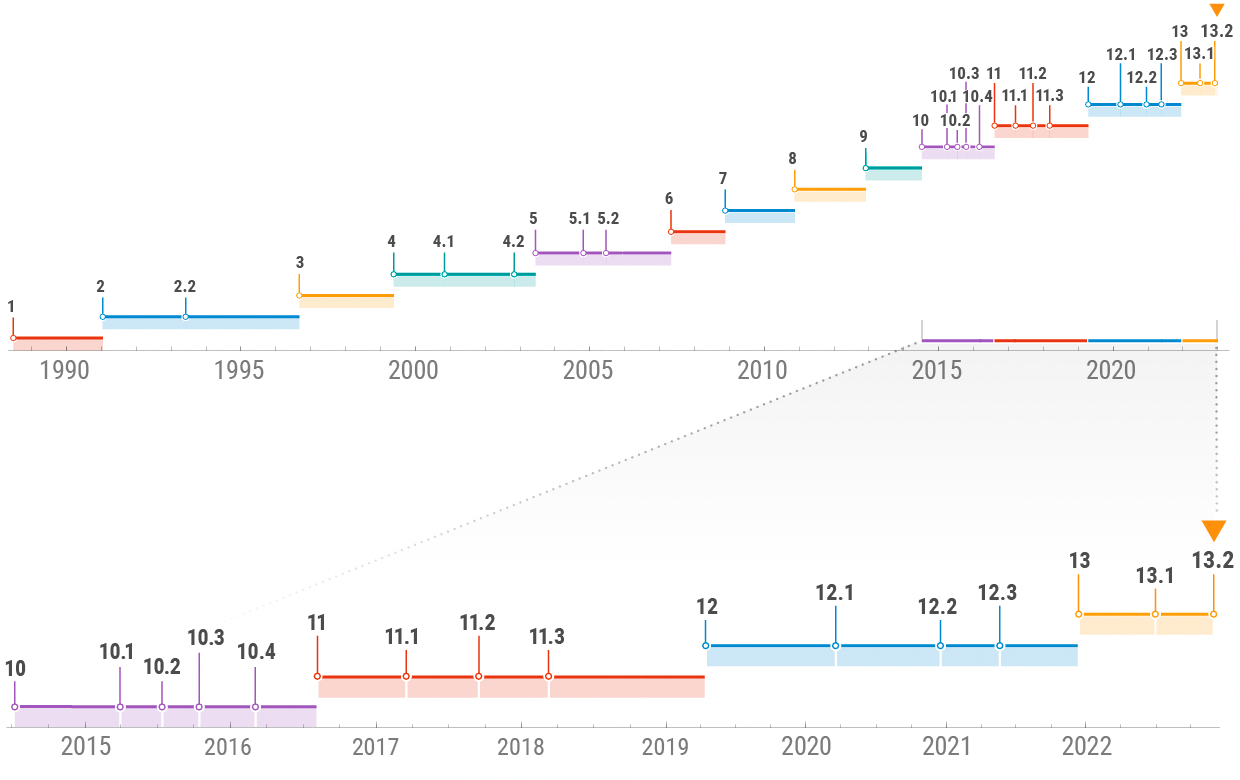
In 2020 it was Variations 12.1 and 12.2; in 2021 Variations 12.3 and 13.0. In late June this 12 months it was Model 13.1. And now we’re releasing Model 13.2. We proceed to have an enormous pipeline of R&D, some quick time period, some medium time period, some long run (like decade-plus). Our purpose is to ship well timed snapshots of the place we’re at—so folks can begin utilizing what we’ve constructed as rapidly as doable.

Model 13.2 is—by our requirements—a reasonably small launch, that principally concentrates on rounding out areas which were underneath improvement for a very long time, in addition to including “polish” to a variety of current capabilities. Nevertheless it’s additionally acquired some “shock” new dramatic effectivity enhancements, and it’s acquired some first hints of main new areas that we’ve got underneath improvement—significantly associated to astronomy and celestial mechanics.

However although I’m calling it a “small launch”, Model 13.2 nonetheless introduces utterly new features into the Wolfram Language, 41 of them—in addition to considerably enhancing 64 current features. And, as standard, we’ve put loads of effort into coherently designing these features, so that they match into the tightly built-in framework we’ve been constructing for the previous 35 years. For the previous a number of years we’ve been following the precept of open code improvement (does anybody else do that but?)—opening up our core software program design conferences as livestreams. Through the Model 13.2 cycle we’ve completed about 61 hours of design livestreams—getting all types of nice real-time suggestions from the neighborhood (thanks, everybody!). And, sure, we’re holding regular at an total common of 1 hour of livestreamed design time per new perform, and rather less than half that per enhanced perform.

Introducing Astro Computation

Astronomy has been a driving pressure for computation for greater than 2000 years (from the Antikythera system on)… and in Model 13.2 it’s coming to Wolfram Language in an enormous means. Sure, the Wolfram Language (and Wolfram|Alpha) have had astronomical information for effectively over a decade. However what’s new now could be astronomical computation totally built-in into the system. In some ways, our astro computation capabilities are modeled on our geo computation ones. However astro is considerably extra sophisticated. Mountains don’t transfer (not less than perceptibly), however planets definitely do. Relativity additionally isn’t necessary in geography, however it’s in astronomy. And on the Earth, latitude and longitude are good normal methods to explain the place issues are. However in astronomy—particularly with every part shifting—describing the place issues are is far more sophisticated. Oh, and there’s the query of the place issues “are,” versus the place issues seem like—due to results starting from light-propagation delays to refraction within the Earth’s environment.

The important thing perform for representing the place astronomical issues are is AstroPosition. Right here’s the place Mars is now:

What does that output imply? It’s very “right here and now” oriented. By default, it’s telling me the azimuth (angle from north) and altitude (angle above the horizon) for Mars from the place Right here says I’m, on the time specified by Now. How can I get a much less “private” illustration of “the place Mars is”? As a result of if even I simply reevaluate my earlier enter now, I’ll get a barely completely different reply, simply due to the rotation of the Earth:

One factor to do is to make use of equatorial coordinates, which can be based mostly on a body centered on the middle of the Earth however not rotating with the Earth. (One path is outlined by the rotation axis of the Earth, the opposite by the place the Solar is on the time of the spring equinox.) The result’s the “astronomer-friendly” proper ascension/declination place of Mars:

And perhaps that’s ok for a terrestrial astronomer. However what if you wish to specify the place of Mars in a means that doesn’t check with the Earth? Then you should utilize the now-standard ICRS body, which is centered on the middle of mass of the Photo voltaic System:

Usually in astronomy the query is mainly “which path ought to I level my telescope in?”, and that’s one thing one needs to specify in spherical coordinates. However significantly if one’s “out and about within the Photo voltaic System” (say fascinated with a spacecraft), it’s extra helpful to have the ability to give precise Cartesian coordinates for the place one is:

And listed here are the uncooked coordinates (by default in astronomical models):

AstroPosition is backed by plenty of computation, and particularly by ephemeris information that covers all planets and their moons, along with different substantial our bodies within the Photo voltaic System:

By the way in which, significantly the primary time you ask for the place of an obscure object, there could also be some delay whereas the mandatory ephemeris will get downloaded. The primary ephemerides we use give information for the interval 2000–2050. However we even have entry to different ephemerides that cowl for much longer intervals. So, for instance, we are able to inform the place Ganymede was when Galileo first noticed it:

We even have place information for greater than 100,000 stars, galaxies, pulsars and different objects—with many extra coming quickly:

Issues get sophisticated in a short time. Right here’s the place of Venus seen from Mars, utilizing a body centered on the middle of Mars:

If we decide a selected level on Mars, then we are able to get the end in azimuth-altitude coordinates relative to the Martian horizon:

One other complication is that in case you’re taking a look at one thing from the floor of the Earth, you’re wanting by means of the environment, and the environment refracts gentle, making the place of the article look completely different. By default, AstroPosition takes account of this whenever you use coordinates based mostly on the horizon. However you’ll be able to swap it off, after which the outcomes might be completely different—and, for instance, for the Solar at sundown, considerably completely different:

After which there’s the velocity of sunshine, and relativity, to consider. Let’s say we need to know the place Neptune “is” now. Properly, will we imply the place Neptune “truly is”, or will we imply “the place we observe Neptune to be” based mostly on gentle from Neptune coming to us? For frames referring to observations from Earth, we’re usually involved with the case the place we embody the “gentle time” impact—and, sure, it does make a distinction:

OK, so AstroPosition—which is the analog of GeoPosition—offers us a solution to characterize the place issues are, astronomically. The following necessary perform to debate is AstroDistance—the analog of GeoDistance.

This provides the present distance between Venus and Mars:

That is the present distance from the place we’re (based on Right here) and the place of the Viking 2 lander on Mars:

That is the space from Right here to the star τ Ceti:

To be extra exact, AstroDistance actually tells us the space from a sure object, to an observer, at a sure native time for the observer (and, sure, the truth that it’s native time issues due to gentle delays):

And, sure, issues are fairly exact. Right here’s the space to the Apollo 11 touchdown website on the Moon, computed 5 occasions with a 1-second pause in between, and proven to 10-digit precision:

This plots the space to Mars for daily within the subsequent 10 years:

One other perform is AstroAngularSeparation, which supplies the angular separation between two objects as seen from a given place. Right here’s the outcome from Jupiter and Saturn (seen from the Earth) over a 20-year span:

The Beginnings of Astro Graphics

Along with with the ability to compute astronomical issues, Model 13.2 contains first steps in visualizing astronomical issues. There’ll be extra on this in subsequent variations. However Model 13.2 already has some highly effective capabilities.

As a primary instance, right here’s part of the sky round Betelgeuse as seen proper now from the place I’m:

Zooming out, one can see extra of the sky:

There are many choices for a way issues needs to be rendered. Right here we’re seeing a practical picture of the sky, with grid strains superimposed, aligned with the equator of the Earth:

And right here we’re seeing a extra whimsical interpretation:

Similar to for maps of the Earth, projections matter. Right here’s a Lambert azimuthal projection of the entire sky:

The blue line exhibits the orientation of the Earth’s equator, the yellow line exhibits the aircraft of the ecliptic (which is mainly the aircraft of the Photo voltaic System), and the pink line exhibits the aircraft of our galaxy (which is the place we see the Milky Approach).

If we need to know what we truly “see within the sky” we want a stereographic projection (on this case centered on the south path):

There’s loads of element within the astronomical information and computations we’ve got (and much more might be coming quickly). So, for instance, if we zoom in on Jupiter we are able to see the positions of its moons (although their disks are too small to be rendered right here):

It’s enjoyable to see how this corresponds to Galileo’s authentic statement of those moons greater than 400 years in the past. That is from Galileo:

The previous typesetting does trigger a little bit hassle:

However the astronomical computation is extra timeless. Listed here are the computed positions of the moons of Jupiter from when Galileo stated he noticed them, in Padua:

And, sure, the outcomes agree!

By the way in which, right here’s one other computation that might be verified quickly. That is the time of most eclipse for an upcoming photo voltaic eclipse:

And right here’s what it’ll appear to be from a selected location proper at the moment:

Dates, Instances and Items: There’s All the time Extra to Do

Dates are sophisticated. Even with none of the problems of relativity that we’ve got to take care of for astronomy, it’s surprisingly troublesome to constantly “identify” occasions. What time zone are you speaking about? What calendar system will you utilize? And so forth. Oh, after which what granularity of time are you speaking about? A day? Per week? A month (no matter meaning)? A second? An instantaneous second (or maybe a single elementary time from our Physics Mission)?

These points come up in what one may think can be trivial features: the brand new RandomDate and RandomTime in Model 13.2. Should you don’t say in any other case, RandomDate will give an instantaneous second of time, in your present time zone, along with your default calendar system, and so on.—randomly picked inside the present 12 months:

However let’s say you need a random date in June 1988. You are able to do that by giving the date object that represents that month:

OK, however let’s say you don’t need an instantaneous of time then, however as a substitute you need a complete day. The brand new possibility DateGranularity permits this:

You may ask for a random time within the subsequent 6 hours:

Or 10 random occasions:

You may as well ask for a random date inside some interval—or assortment of intervals—of dates:

And, evidently, we accurately pattern uniformly over any assortment of intervals:

One other space of just about arbitrary complexity is models. And over the course of a few years we’ve systematically solved downside after downside in supporting mainly each form of unit that’s in use (now greater than 5000 base varieties). However one holdout has concerned temperature. In physics textbooks, it’s conventional to rigorously distinguish absolute temperatures, measured in kelvins, from temperature scales, like levels Celsius or Fahrenheit. And that’s necessary, as a result of whereas absolute temperatures may be added, subtracted, multiplied and so on. similar to different models, temperature scales on their very own can’t. (Multiplying by 0° C to get 0 for one thing like an quantity of warmth can be very improper.) Then again, variations in temperature—even measured in Celsius—may be multiplied. How can all this be untangled?

In earlier variations we had a complete completely different form of unit (or, extra exactly, completely different bodily amount dimension) for temperature variations (a lot as mass and time have completely different dimensions). However now we’ve acquired a greater answer. We’ve mainly launched new models—however nonetheless “temperature-dimensioned” ones—that characterize temperature variations. And we’ve launched a brand new notation (a little bit Δ subscript) to point them:

Should you take a distinction between two temperatures, the outcome may have temperature-difference models:

However in case you convert this to an absolute temperature, it’ll simply be in extraordinary temperature models:

And with this unscrambled, it’s truly doable to do arbitrary arithmetic even on temperatures measured on any temperature scale—although the outcomes additionally come again as absolute temperatures:

It’s value understanding that an absolute temperature may be transformed both to a temperature scale worth, or a temperature scale distinction:

All of this implies you can now use temperatures on any scale in formulation, and so they’ll simply work:

Dramatically Sooner Polynomial Operations

Nearly any algebraic computation finally ends up by some means involving polynomials. And polynomials have been a well-optimized a part of Mathematica and the Wolfram Language for the reason that starting. And in reality, little has wanted to be up to date within the basic operations we do with them in additional than 1 / 4 of a century. However now in Model 13.2—because of new algorithms and new information buildings, and new methods to make use of trendy laptop {hardware}—we’re updating some core polynomial operations, and making them dramatically sooner. And, by the way in which, we’re getting some new polynomial performance as effectively.

Here’s a product of two polynomials, expanded out:

Factoring polynomials like that is just about instantaneous, and has been ever since Model 1:

However now let’s make this greater:

There are 999 phrases within the expanded polynomial:

Factoring this isn’t a straightforward computation, and in Model 13.1 takes about 19 seconds:

However now, in Model 13.2, the identical computation takes 0.3 seconds—practically 60 occasions sooner:

It’s fairly uncommon that something will get 60x sooner. However that is a type of instances, and in reality for nonetheless bigger polynomials, the ratio will steadily improve additional. However is that this simply one thing that’s solely related for obscure, huge polynomials? Properly, no. Not least as a result of it seems that huge polynomials present up “underneath the hood” in all types of necessary locations. For instance, the innocuous-seeming object

may be manipulated as an algebraic quantity, however with minimal polynomial:

Along with factoring, Model 13.2 additionally dramatically will increase the effectivity of polynomial resultants, GCDs, discriminants, and so on. And all of this makes doable a transformative replace to polynomial linear algebra, i.e. operations on matrices whose components are (univariate) polynomials.

Right here’s a matrix of polynomials:

And right here’s an influence of the matrix:

And the determinant of this:

In Model 13.1 this didn’t look practically as good; the outcome comes out unexpanded as:

Each measurement and velocity are dramatically improved in Model 13.2. Right here’s a bigger case—the place in 13.1 the computation takes greater than an hour, and the outcome has a staggering leaf rely of 178 billion

however in Model 13.2 it’s 13,000 occasions sooner, and 60 million occasions smaller:

Polynomial linear algebra is used “underneath the hood” in a outstanding vary of areas, significantly in dealing with linear differential equations, distinction equations, and their symbolic options. And in Model 13.2, not solely polynomial MatrixPower and Det, but additionally LinearSolve, Inverse, RowReduce, MatrixRank and NullSpace have been dramatically sped up.

Along with the dramatic velocity enhancements, Model 13.2 additionally provides a polynomial characteristic for which I, for one, occur to have been ready for greater than 30 years: multivariate polynomial factoring over finite fields:

Certainly, wanting in our archives I discover many requests stretching again to not less than 1990—from fairly a variety of individuals—for this functionality, although, charmingly, a 1991 inside be aware states:

Yup, that was proper. However 31 years later, in Model 13.2, it’s completed!

Integrating Exterior Neural Nets

The Wolfram Language has had built-in neural internet expertise since 2015. Generally that is robotically used inside different Wolfram Language features, like ImageIdentify, SpeechRecognize or Classify. However you too can construct your individual neural nets utilizing the symbolic specification language with features like NetChain and NetGraph—and the Wolfram Neural Web Repository supplies a regularly up to date supply of neural nets you can instantly use, and modify, within the Wolfram Language.

However what if there’s a neural internet on the market that you simply simply need to run from inside the Wolfram Language, however don’t must have represented in modifiable (or trainable) symbolic Wolfram Language kind—such as you may run an exterior program executable? In Model 13.2 there’s a brand new assemble NetExternalObject that lets you run educated neural nets “from the wild” in the identical built-in framework used for precise Wolfram-Language-specified neural nets.

NetExternalObject to this point helps neural nets which were outlined within the ONNX neural internet change format, which may simply be generated from frameworks like PyTorch, TensorFlow, Keras, and so on. (in addition to from Wolfram Language). One can get a NetExternalObject simply by importing an .onnx file. Right here’s an instance from the online:

If we “open up” the abstract for this object we see what primary tensor construction of enter and output it offers with:

However to really use this community we’ve got to arrange encoders and decoders appropriate for the precise operation of this specific community—with the actual encoding of pictures that it expects:

Now we simply must run the encoder, the exterior community and the decoder—to get (on this case) a cartoonized Mount Rushmore:

Usually the “wrapper code” for the NetExternalObject might be a bit extra sophisticated than on this case. However the built-in NetEncoder and NetDecoder features sometimes present an excellent begin, and basically the symbolic construction of the Wolfram Language (and its built-in capacity to characterize pictures, video, audio, and so on.) makes the method of importing typical neural nets “from the wild” surprisingly easy. And as soon as imported, such neural nets can be utilized immediately, or as parts of different features, anyplace within the Wolfram Language.

Displaying Giant Bushes, and Making Extra

We first launched timber as a basic construction in Model 12.3, and we’ve been enhancing them ever since. In Model 13.1 we added many choices for figuring out how timber are displayed, however in Model 13.2 we’re including one other, crucial one: the flexibility to elide massive subtrees.

Right here’s a size-200 random tree with each department proven:

And right here’s the identical tree with each node being instructed to show a most of three youngsters:

And, truly, tree elision is handy sufficient that in Model 13.2 we’re doing it by default for any node that has greater than 10 youngsters—and we’ve launched the worldwide $MaxDisplayedChildren to find out what that default restrict needs to be.

One other new tree characteristic in Model 13.2 is the flexibility to create timber out of your file system. Right here’s a tree that goes down 3 listing ranges from my Wolfram Desktop set up listing:

Calculus & Its Generalizations

Is there nonetheless extra to do in calculus? Sure! Generally the purpose is, for instance, to unravel extra differential equations. And typically it’s to unravel current ones higher. The purpose is that there could also be many various doable types that may be given for a symbolic answer. And sometimes the types which can be best to generate aren’t those which can be most helpful or handy for subsequent computation, or the simplest for a human to know.

In Model 13.2 we’ve made dramatic progress in bettering the type of options that we give for essentially the most sorts of differential equations, and methods of differential equations.

Right here’s an instance. In Model 13.1 that is an equation we may clear up symbolically, however the answer we give is lengthy and sophisticated:

However now, in 13.2, we instantly give a way more compact and helpful type of the answer:

The simplification is usually much more dramatic for methods of differential equations. And our new algorithms cowl a full vary of differential equations with fixed coefficients—that are what go by the identify LTI (linear time-invariant) methods in engineering, and are used fairly universally to characterize electrical, mechanical, chemical, and so on. methods.

Along with streamlining “on a regular basis calculus”, we’re additionally pushing on some frontiers of calculus, like fractional calculus. In Model 13.1 we launched symbolic fractional differentiation, with features like FractionalD. In Model 13.2 we now even have numerical fractional differentiation, with features like NFractionalD, right here proven getting the ½^th spinoff of Sin[x]:

In Model 13.1 we launched symbolic options of fractional differential equations with fixed coefficients; now in Model 13.2 we’re extending this to asymptotic options of fractional differential equations with each fixed and polynomial coefficients. Right here’s an Ethereal-like differential equation, however generalized to the fractional case with a Caputo fractional spinoff:

Evaluation of Cluster Evaluation

The Wolfram Language has had primary built-in assist for cluster evaluation for the reason that mid-2000s. However in newer occasions—with elevated sophistication from machine studying—we’ve been including increasingly subtle types of cluster evaluation. Nevertheless it’s one factor to do cluster evaluation; it’s one other to research the cluster evaluation one’s completed, to attempt to higher perceive what it means, the right way to optimize it, and so on. In Model 13.2 we’re each including the perform ClusteringMeasurements to do that, in addition to including extra choices for cluster evaluation, and enhancing the automation we’ve got for technique and parameter choice.

Let’s say we do cluster evaluation on some information, asking for a sequence of various numbers of clusters:

Which is the “greatest” variety of clusters? One measure of that is to compute the “silhouette rating” for every doable clustering, and that’s one thing that ClusteringMeasurements can now do:

As is pretty typical in statistics-related areas, there are many completely different scores and standards one can use—ClusteringMeasurements helps all kinds of them.

Chess as Computable Knowledge

Our purpose with Wolfram Language is to make as a lot as doable computable. Model 13.2 provides yet one more area—chess—supporting import of the FEN and PGN chess codecs:

PGN recordsdata sometimes include many video games, every represented as a listing of FEN strings. This counts the variety of video games in a selected PGN file:

Right here’s the primary sport within the file:

Given this, we are able to now use Wolfram Language’s video capabilities to make a video of the sport:

Controlling Runaway Computations

Again in 1979 once I began constructing SMP—the forerunner to the Wolfram Language—I did one thing that to some folks appeared very daring, even perhaps reckless: I arrange the system to basically do “infinite analysis”, that’s, to proceed utilizing no matter definitions had been given till nothing extra might be completed. In different phrases, the method of analysis would all the time go on till a set level was reached. “However what occurs if x doesn’t have a price, and also you say x = x + 1?” folks would ask. “Gained’t the system blow up in that case?” Properly, in some sense sure. However I took a calculated gamble that the advantages of infinite analysis for extraordinary computations that folks truly need to do would vastly outweigh any doable points with what appeared like “pointless nook instances” reminiscent of x = x + 1. Properly, 43 years later I believe I can say with some confidence that that gamble labored out. The idea of infinite analysis—mixed with the symbolic construction of the Wolfram Language—has been a supply of super energy, and most customers merely by no means run into, and by no means have to consider, the x = x + 1 “nook case”.

Nonetheless, in case you sort x = x + 1 the system clearly has to do one thing. And in a way the purest factor to do would simply be to proceed computing ceaselessly. However 34 years in the past that led to a quite disastrous downside on precise computer systems—and in reality nonetheless does as we speak. As a result of basically this sort of repeated analysis is a recursive course of, that finally needs to be carried out utilizing the decision stack arrange for each occasion of a program by the working system. However the way in which working methods work (nonetheless!) is to allocate solely a set quantity of reminiscence for the stack—and if that is overrun, the working system will merely make your program crash (or, in earlier occasions, the working system itself may crash). And this meant that ever since Model 1, we’ve wanted to have a restrict in place on infinite analysis. In early variations we tried to present the “results of the computation to this point”, wrapped in Maintain. Again in Model 10, we began simply returning a held model of the unique expression:

However even that is in a way not secure. As a result of with different infinite definitions in place, one can find yourself with a scenario the place even attempting to return the held kind triggers further infinite computational processes.

In latest occasions, significantly with our exploration of multicomputation, we’ve determined to revisit the query of the right way to restrict infinite computations. At some theoretical degree, one may think explicitly representing infinite computations utilizing issues like transfinite numbers. However that’s fraught with issue, and manifest undecidability (“Is that this infinite computation output actually the identical as that one?”, and so on.) However in Model 13.2, as the start of a brand new, “purely symbolic” strategy to “runaway computation” we’re introducing the assemble TerminatedEvaluation—that simply symbolically represents, because it says, a terminated computation.

So right here’s what now occurs with x = x + 1:

A notable characteristic of that is that it’s “independently encapsulated”: the termination of 1 a part of a computation doesn’t have an effect on others, in order that, for instance, we get:

There’s an advanced relation between terminated evaluations and lazy analysis, and we’re engaged on some attention-grabbing and probably highly effective new capabilities on this space. However for now, TerminatedEvaluation is a crucial assemble for bettering the “security” of the system within the nook case of runaway computations. And introducing it has allowed us to repair what appeared for a few years like “theoretically unfixable” points round complicated runaway computations.

TerminatedEvaluation is what you run into in case you hit system-wide “guard rails” like $RecursionLimit. However in Model 13.2 we’ve additionally tightened up the dealing with of explicitly requested aborts—by including the brand new possibility PropagateAborts to CheckAbort. As soon as an abort has been generated—both immediately by utilizing Abort[ ], or as the results of one thing like TimeConstrained[ ] or MemoryConstrained[ ]—there’s a query of how far that abort ought to propagate. By default, it’ll propagate all the way in which up, so your complete computation will find yourself being aborted. However ever since Model 2 (in 1991) we’ve had the perform CheckAbort, which checks for aborts within the expression it’s given, then stops additional propagation of the abort.

However there was all the time loads of trickiness across the query of issues like TimeConstrained[ ]. Ought to aborts generated by these be propagated the identical means as Abort[ ] aborts or not? In Model 13.2 we’ve now cleaned all of this up, with an express possibility PropagateAborts for CheckAbort. With PropagateAborts→True all aborts are propagated, whether or not initiated by Abort[ ] or TimeConstrained[ ] or no matter. PropagateAborts→False propagates no aborts. However there’s additionally PropagateAborts→Computerized, which propagates aborts from TimeConstrained[ ] and so on., however not from Abort[ ].

But One other Little Listing Operate

In our endless strategy of extending and sharpening the Wolfram Language we’re continually looking out for “lumps of computational work” that folks repeatedly need to do, and for which we are able to create features with easy-to-understand names. Today we frequently prototype such features within the Wolfram Operate Repository, then additional streamline their design, and ultimately implement them within the everlasting core Wolfram Language. In Model 13.2 simply two new primary list-manipulation features got here out of this course of: PositionLargest and PositionSmallest.

We’ve had the perform Place since Model 1, in addition to Max. However one thing I’ve typically discovered myself needing to do through the years is to mix these to reply the query: “The place is the max of that listing?” In fact it’s not onerous to do that within the Wolfram Language—Place[list, Max[list]] mainly does it. However there are some edge instances and extensions to consider, and it’s handy simply to have one perform to do that. And, what’s extra, now that we’ve got features like TakeLargest, there’s an apparent, constant identify for the perform: PositionLargest. (And by “apparent”, I imply apparent after you hear it; the archive of our livestreamed design evaluation conferences will reveal that—as is so typically the case—it truly took us fairly some time to decide on the “apparent”.)

Right here’s PositionLargest and in motion:

And, sure, it has to return a listing, to take care of “ties”:

Graphics, Picture, Graph, …? Inform It from the Body Colour

All the pieces within the Wolfram Language is a symbolic expression. However completely different symbolic expressions are displayed otherwise, which is, after all, very helpful. So, for instance, a graph isn’t displayed within the uncooked symbolic kind

however quite as a graph:

However let’s say you’ve acquired a complete assortment of visible objects in a pocket book. How will you inform what they “actually are”? Properly, you’ll be able to click on them, after which see what coloration their borders are. It’s refined, however I’ve discovered one rapidly will get used to noticing not less than the sorts of objects one generally makes use of. And in Model 13.2 we’ve made some further distinctions, notably between pictures and graphics.

So, sure, the article above is a Graph—and you may inform that as a result of it has a purple border whenever you click on it:

This can be a Graphics object, which you’ll inform as a result of it’s acquired an orange border:

And right here, now, is an Picture object, with a light-weight blue border:

For some issues, coloration hints simply don’t work, as a result of folks can’t bear in mind which coloration means what. However for some cause, including coloration borders to visible objects appears to work very effectively; it supplies the fitting degree of hinting, and the truth that one typically sees the colour when it’s apparent what the article is helps cement a reminiscence of the colour.

In case you’re questioning, there are some others already in use for borders—and extra to return. Bushes are inexperienced (although, sure, ours by default develop down). Meshes are brown:

Brighter, Higher Syntax Coloring

How will we make it as simple as doable to sort appropriate Wolfram Language code? This can be a query we’ve been engaged on for years, regularly inventing increasingly mechanisms and options. In Model 13.2 we’ve made some small tweaks to a mechanism that’s truly been within the system for a few years, however the adjustments we’ve made have a considerable impact on the expertise of typing code.

One of many huge challenges is that code is typed “linearly”—basically (other than 2D constructs) from left to proper. However (similar to in pure languages like English) the that means is outlined by a extra hierarchical tree construction. And one of many points is to know the way one thing you typed matches into the tree construction.

One thing like that is visually apparent fairly regionally within the “linear” code you typed. However typically what defines the tree construction is kind of distant. For instance, you may need a perform with a number of arguments which can be every massive expressions. And whenever you’re taking a look at one of many arguments it is probably not apparent what the general perform is. And a part of what we’re now emphasizing extra strongly in Model 13.2 is dynamic highlighting that exhibits you “what perform you’re in”.

It’s highlighting that seems whenever you click on. So, for instance, that is the highlighting you get clicking at a number of completely different positions in a easy expression:

Right here’s an instance “from the wild” exhibiting you that in case you sort on the place of the cursor, you’ll be including an argument to the ContourPlot perform:

However now let’s click on in a distinct place:

Right here’s a smaller instance:

Discover that we’re highlighting each the enclosing grouping {…} and the enclosing perform head.

We’ve had the fundamental functionality for this sort of highlighting for practically a decade. However in Model 13.2 we’re making it a lot bolder, and we’ve subtly tweaked what highlighting exhibits up when. This will likely look like a element, however I, for instance, have discovered it fairly transformative in the way in which that I truly sort code.

Previously I typically discovered myself multiclicking to determine the construction of the code. However now I simply must click on and the highlighting is vivid sufficient to be instantly apparent, even when it’s fairly distant within the linear rendering of the code.

It’s additionally necessary that the highlighting colours for perform heads and for grouping constructs at the moment are far more distinct. Previously, they have been each shades of inexperienced, which have been onerous to differentiate and perceive. With the Model 13.2 colours one rapidly will get used to how issues are arrange, and it’s simple to get a way of the construction of an expression. And having these two colours (versus extra, or fewer) appears to be about proper by way of giving info, however not giving a lot that it’s onerous to assimilate.

Consumer Interface Conveniences

We first launched the pocket book interface in Model 1 again in 1988. And already in that model we had most of the present options of notebooks—like cells and cell teams, cell kinds, and so on. However over the previous 34 years we’ve been persevering with to tweak and polish the pocket book interface to make it ever smoother to make use of.

In Model 13.2 we’ve got some minor however handy additions. We’ve had the Divide Cell menu merchandise (cmdshiftD) for greater than 30 years. And the way in which it’s all the time labored is that you simply click on the place you need a cell to be divided. In the meantime, we’ve all the time had the flexibility to place a number of Wolfram Language inputs right into a single cell. And whereas typically it’s handy to sort code that means, or import it from elsewhere like that, it makes higher use of all our pocket book and cell capabilities if every unbiased enter is in its personal cell. And now in Model 13.2 Divide Cell could make it like that, analyzing multiline inputs to divide them between full inputs that happen on completely different strains:

Equally, in case you’re coping with textual content as a substitute of code, Divide Cell will now divide at express line breaks—that may correspond to paragraphs.

In a very completely different space, Model 13.1 added a brand new default toolbar for notebooks, and in Model 13.2 we’re starting the method of steadily including options to this toolbar. The primary apparent characteristic that’s been added is a brand new interactive software for altering frames in cells. It’s a part of the Cell Look merchandise within the toolbar:

Simply click on a aspect of the body type widget and also you’ll get a software to edit that body type—and also you’ll instantly see any adjustments mirrored within the pocket book:

If you wish to edit all the perimeters, you’ll be able to lock the settings along with:

Cell frames have all the time been a helpful mechanism for delineating, highlighting or in any other case annotating cells in notebooks. However prior to now it’s been comparatively troublesome to customise them past what’s within the stylesheet you’re utilizing. With the brand new toolbar characteristic in Model 13.2 we’ve made it very simple to work with cell frames, making it practical for customized cell frames to turn out to be a routine a part of pocket book content material.

Mixing Compiled and Evaluated Code

We’ve labored onerous to have code you write within the Wolfram Language instantly run effectively. However by taking the additional one-time effort to invoke the Wolfram Language compiler—telling it extra particulars about the way you count on to make use of your code— you’ll be able to typically make your code run extra effectively, and typically dramatically so. In Model 13.2 we’ve been persevering with the method of streamlining the workflow for utilizing the compiler, and for unifying code that’s arrange for compilation, and code that’s not.

The first work you need to do as a way to make the perfect use of the Wolfram Language compiler is in specifying varieties. One of many necessary options of the Wolfram Language basically is {that a} image x can simply as effectively be an integer, a listing of complicated numbers or a symbolic illustration of a graph. However the principle means the compiler provides effectivity is by with the ability to assume that x is, say, all the time going to be an integer that matches right into a 64-bit laptop phrase.

The Wolfram Language compiler has a complicated symbolic language for specifying varieties. Thus, for instance

is a symbolic specification for the kind of a perform that takes two 64-bit integers as enter, and returns a single one. TypeSpecifier[ ... ] is a symbolic assemble that doesn’t consider by itself, and can be utilized and manipulated symbolically. And it’s the identical story with Typed[ ... ], which lets you annotate an expression to say what sort it needs to be assumed to be.

However what if you wish to write code which may both be evaluated within the extraordinary means, or fed to the compiler? Constructs like Typed[ ... ] are for everlasting annotation. In Model 13.2 we’ve added TypeHint which lets you give a touch that can be utilized by the compiler, however might be ignored in extraordinary analysis.

This compiles a perform assuming that its argument x is an 8-bit integer:

By default, the 100 right here is assumed to be represented as a 64-bit integer. However with a kind trace, we are able to say that it too needs to be represented as an 8-bit integer:

150 doesn’t slot in an 8-bit integer, so the compiled code can’t be used:

However what’s related right here is that the perform we compiled can be utilized not just for compilation, but additionally in extraordinary analysis, the place the TypeHint successfully simply “evaporates”:

Because the compiler develops, it’s going to have the ability to do increasingly sort inferencing by itself. Nevertheless it’ll all the time be capable of get additional if the person offers it some hints. For instance, if x is a 64-bit integer, what sort needs to be assumed for x^x? There are definitely values of x for which x^x received’t slot in a 64-bit integer. However the person may know these received’t present up. And to allow them to give a kind trace that claims that the x^x needs to be assumed to slot in a 64-bit integer, and this may permit the compiler to do far more with it.

It’s value declaring that there are all the time going to be limitations to sort inferencing, as a result of, in a way, inferring varieties requires proving theorems, and there may be theorems which have arbitrarily lengthy proofs, or no proofs in any respect in a sure axiomatic system. For instance, think about asking whether or not the kind of a zero of the Riemann zeta perform has a sure imaginary half. To reply this, the kind inferencer must clear up the Riemann speculation. But when the person simply needed to imagine the Riemann speculation, they might—not less than in precept—use TypeHint.

TypeHint is a wrapper meaning one thing to the compiler, however “evaporates” in extraordinary analysis. Model 13.2 provides IfCompiled, which helps you to explicitly delineate code that needs to be used with the compiler, and code that needs to be utilized in extraordinary analysis. That is helpful when, for instance, extraordinary analysis can use a complicated built-in Wolfram Language perform, however compiled code might be extra environment friendly if it successfully builds up related performance from lower-level primitives.

In its easiest kind FunctionCompile permits you to take an express pure perform and make a compiled model of it. However what you probably have a perform the place you’ve already assigned downvalues to it, like:

Now in Model 13.2 you should utilize the brand new DownValuesFunction wrapper to present a perform like this to FunctionCompile:

That is necessary as a result of it permits you to arrange a complete community of definitions utilizing := and so on., then have them robotically be fed to the compiler. Generally, you should utilize DownValuesFunction as a wrapper to tag any use of a perform you’ve outlined elsewhere. It’s considerably analogous to the KernelFunction wrapper that you should utilize to tag built-in features, and specify what varieties you need to assume for them in code that you simply’re feeding to the compiler.

Packaging Giant-Scale Compiled Code

Let’s say you’re constructing a considerable piece of performance that may embody compiled Wolfram Language code, exterior libraries, and so on. In Model 13.2 we’ve added capabilities to make it simple to “bundle up” such performance, and for instance deploy it as a distributable paclet.

For instance of what may be completed, this installs a paclet referred to as GEOSLink that features the GEOS exterior library and compiler-based performance to entry this:

Now that the paclet is put in, we are able to use a file from it to arrange a complete assortment of features which can be outlined within the paclet:

Given the code within the paclet we are able to now simply begin calling features that use the GEOS library:

It’s fairly nontrivial that this “simply works”. As a result of for it to work, the system has to have been instructed to load and initialize the GEOS library, in addition to convert the Wolfram Language polygon geometry to a kind appropriate for GEOS. The returned outcome can also be nontrivial: it’s basically a deal with to information that’s contained in the GEOS library, however being memory-managed by the Wolfram Language system. Now we are able to take this outcome, and name a GEOS library perform on it, utilizing the Wolfram Language binding that’s been outlined for that perform:

This will get the outcome “again from GEOS” into pure Wolfram Language kind:

How does all this work? This goes to the listing for the put in GEOSLink paclet on my system:

There’s a subdirectory referred to as LibraryResources that comprises dynamic libraries appropriate for my laptop system:

The libgeos libraries are the uncooked exterior GEOS libraries “from the wild”. The GEOSLink library is a library that was constructed by the Wolfram Language compiler from Wolfram Language code that defines the “glue” for interfacing between the GEOS library and the Wolfram Language:

What’s all this? It’s all based mostly on new performance in Model 13.2. And finally what it’s doing is to create a CompiledComponent assemble (which is a brand new factor in Model 13.2). A CompiledComponent assemble represents a bundle of compilable performance with components like "Declarations", "InstalledFunctions", "LibraryFunctions", "LoadingEpilogs" and "ExternalLibraries". And in a typical case—just like the one proven right here—one creates (or provides to) a CompiledComponent utilizing DeclareCompiledComponent.

Right here’s an instance of a part of what’s added by DeclareCompiledComponent:

First there’s a declaration of an exterior (on this case GEOS) library perform, giving its sort signature. Then there’s a declaration of a compilable Wolfram Language perform GEOSUnion that immediately calls the GEOSUnion perform within the exterior library, defining it to take a sure memory-managed information construction as enter, and return a equally memory-managed object as output.

From this supply code, all you do to construct an precise library is use BuildCompiledComponent. And given this library you can begin calling exterior GEOS features immediately from top-level Wolfram Language code, as we did above.

However the CompiledComponent object does one thing else as effectively. It additionally units up every part you want to have the ability to write compilable code that calls the identical features as you’ll be able to inside the constructed library.

The underside line is that with all the brand new performance in Model 13.2 it’s turn out to be dramatically simpler to combine compiled code, exterior libraries and so on. and to make them conveniently distributable. It’s a reasonably outstanding simplification of what was beforehand a time-consuming and sophisticated software program engineering problem. And it’s good instance of how highly effective it may be to arrange symbolic specs within the Wolfram Language after which use our compiler expertise to robotically create and deploy code outlined by them.

And Extra…

Along with all of the issues we’ve mentioned, there are different updates and enhancements which have arrived within the six months since Model 13.1 was launched. A notable instance is that there have been no fewer than 241 new features added to the Wolfram Operate Repository throughout that point, offering particular add-on performance in a complete vary of areas:

However inside the core Wolfram Language itself, Model 13.2 additionally provides plenty of little new capabilities, that polish and spherical out current performance. Listed here are some examples:

Parallelize now helps computerized parallelization of a wide range of new features, significantly associated to associations.

Blurring now joins DropShadowing as a 2D graphics impact.

MeshRegion, and so on. can now retailer vertex coloring and vertex normals to permit enhanced visualization of areas.

RandomInstance does a lot better at rapidly discovering non-degenerate examples of geometric scenes that fulfill specified constraints.

ImageStitch now helps stitching pictures onto spherical and cylindrical canvases.

Capabilities like Definition and Clear that function on symbols now constantly deal with lists and string patterns.

FindShortestTour has a direct solution to return particular person options of the outcome, quite than all the time packaging them collectively in a listing.

PersistentSymbol and LocalSymbol now permit reassignment of components utilizing features like AppendTo.

SystemModelMeasurements now offers diagnostics reminiscent of rise time and overshoot for SystemModel management methods.

Import of OSM (OpenStreetMap) and GXF geo codecs at the moment are supported.