Yardsticks to Metric Tensor Fields
[ad_1]
I requested myself why completely different scientists perceive the identical factor seemingly otherwise, particularly the idea of a metric tensor. If we ask a topologist, a classical geometer, an algebraist, a differential geometer, and a physicist “What’s a metric?” then we get 5 completely different solutions. I imply it’s all about distances, isn’t it? “Sure” remains to be the reply and all do really imply the identical factor. It’s their perspective that’s completely different. This text is meant to elucidate how.
The picture exhibits medieval requirements of comparability at a church in Regensburg, Germany, Schuh (shoe), Elle (ulna), and Klafter.
Topology
The topologist has in all probability the simplest idea. A metric is a property of sure topological areas, metric areas. It signifies that the topological area is supplied with a yardstick. A perform that measures distances. The circumstances are clear:
Symmetry
We don’t hassle whether or not we measure from proper to left or from left to proper.
Constructive Definiteness
The gap isn’t destructive, and 0 if and provided that there isn’t a distance between our factors, i.e. it’s the identical level. Sounds foolish, however there are certainly unique topological areas wherein this isn’t a triviality. We simply don’t wish to hassle about these pathological examples.
Triangle Inequality
If we’re going from one level to a different and making a cease at a 3rd level that’s not in our direct approach, then it’s a detour.
All people will perceive that this can be a passable description of what our yardstick is meant to do.
Classical Geometry
Not so the classical geometer! He doesn’t care about distances. His enterprise is comparisons. No, not shorter or longer. His view is how typically one distance matches into one other distance. One might argue that that is nonetheless the idea of a yardstick: how typically does a yard match right into a distance? Nevertheless, the distinction is refined. The classical geometer doesn’t wish to outline a unit, be it a yard or a meter. He at all times compares any two lengths and tells us the quotient of them, e.g. the golden ratio is outlined by
$$
dfrac{a+b}{a}=dfrac{a}{b}quadLongleftrightarrowquad a^2-b^2=ab.
$$
The traditional Greeks didn’t solely cope with distances. If we take a look at the trigonometric features, particularly quotients of two lengths once more, we get to the opposite necessary measure in classical geometry: angles and therewith triangles, ideally proper ones. We now have to contemplate instructions, too.
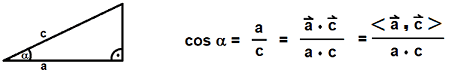
Angles are clearly associated to the multiplication of vectors, and that calls for two different necessary circumstances, the distributive legal guidelines.
Additions
##langle vec{a}+vec{b},vec{c}rangle=langle vec{a},vec{c} rangle +langle vec{b},vec{c} rangle## and ##langle vec{a},vec{b}+vec{c} rangle =langle vec{a},vec{b} rangle +langle vec{a},vec{c} rangle##
Stretches and Compressions
i.e. Scalar Multiples
## alpha langle vec{a},vec{b} rangle =langle alpha vec{ a},vec{b} rangle= langle vec{a},alpha vec{b} rangle##
If we now outline a size by
$$
|vec{a}| :=sqrt{langle vec{a},vec{a} rangle}=sqrt{sum_{ok=1}^n a_k^2},
$$
we get a metric within the topological sense
$$
d(vec{a},vec{b}):=|vec{a}-vec{b}|=sqrt{sum_{ok=1}^n (a_k-b_k)^2}.
$$
and an angle
$$
cos(sphericalangle(vec{a},vec{b}))=dfrac{langle vec{a},vec{b} rangle}{|vec{a}|cdot |vec{b}|}= dfrac{sum_{ok=1}^na_kb_k}{sqrt{sum_{ok=1}^n a_k^2}sqrt{sum_{ok=1}^n b_k^2}}.
$$
Summary Algebra
An algebraist is within the buildings, not a lot in coordinates, so we outline a metric tensor by the properties above slightly than coordinates. A metric tensor for a vector area ##V## is subsequently merely a component of ##V^*otimes V^*.## Nicely, that is true, quick, and doesn’t assist us in any respect. What we wish to outline is an internal product ##langle , . ,, , ,, . , rangle .## That, at its core, is a symmetric, constructive particular, bilinear mapping
$$
g, : ,V occasions V longrightarrow mathbb{R}
$$
Such a mapping will be written as a matrix ##G,## i.e. ##g(vec{a},vec{b})=vec{a}cdot G cdotvec{b}.## We have now thought-about ##g(vec{a},vec{b})=vec{a}cdot operatorname{Id}cdotvec{b}## to date, the place ##operatorname{Id}## is the identification matrix. Nevertheless, there isn’t a motive to limit ourselves to the identification matrix. Any constructive particular matrix ##G## will do. That is mainly saying ##gin V^*otimes V^*.## In a while, we are going to even drop this situation and solely demand that ##G## is non-degenerate, i.e. that for each vector ##vec{a}neq vec{0}## there’s a vector ##vec{b}## such that ##g(vec{a},vec{b})neq vec{0}.## With ##G=operatorname{Id}## we have now a particular instance of a vector area ##V=mathbb{R}^n## that offers the development a which means.
The metric tensor ##g_pin V^*otimes V^*## above an affine level area ##A={p}+V## with translation area ##V## is a mapping that assigns to ##{p}## a symmetric, constructive particular, bilinear mapping ##g_p.## Size, distance and angle for ##vec{a},vec{b}in V ## at the moment are given as
start{align*}
|vec{a}|_p&=sqrt{g_p(vec{a},vec{a})}
d_p(vec{a},vec{b})&=|vec{a}-vec{b}|_p
cos(sphericalangle_p(vec{a},vec{b}))&=dfrac{g_p(vec{a},vec{b})}{|vec{a}|_pcdot|vec{b}|_p}
finish{align*}
If we have now an affine linear monomorphism ##varphi , : ,{p}+U rightarrowtail {varphi(p)}+V## then any metric tensor on ##{varphi(p)}+V## defines a metric tensor on ##{p}+U## by the definition
$$(varphi^* g)_p(vec{u}_1,vec{u}_2):=g_{varphi(p)}(varphi_*(vec{u}_1),varphi_*(vec{u}_2)).$$
This pullback, or likewise the truth that ##g_pin T(V^*),## is the explanation the algebraist calls the metric tensor contravariant: Given one other monomorphism ##psi , : ,{varphi(p)} +V rightarrowtail {psi(varphi(p))}+W## then ##(psi circvarphi)^*(g_p)=g_{varphi(p)}circ g_{psi(varphi(p))}=(varphi^*circ psi^*)(g_p).## This alteration of order means for mathematicians contravariance. (Consideration: physicists name it covariant for various causes, see under!)
You will need to discover that each one three portions rely on the purpose ##p.##
Manifolds
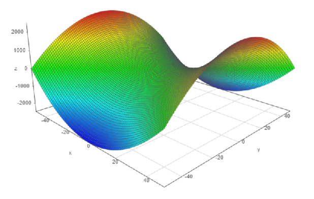
All the above has been slightly theoretical to date. Certain, the topologist might clarify our yardstick and the traditional Greeks have been actually glorious in Euclidean geometry. However it isn’t till we meet the differential geometer and the physicist to inform us one thing about the true world, the non-Euclidean realities, and the truth that the algebraist’s perspective was not utterly irrelevant. They deal e.g. with saddles:
If we improve the decision, rotate the saddle a bit, and eventually zoom in, and focus on that small marked sq.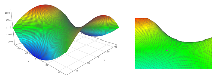
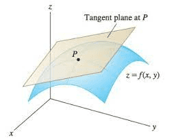
then we will faux that this can be a small flat aircraft that represents the tangent area sooner or later inside the sq.. The smaller we select our sq.. the smaller the error in any calculations because of curvature. After which we will do the identical with any neighboring sq.. We solely demand that the calculations of any overlapping elements should be the identical, for brief: charts, an atlas, and an internal product on ##T_pM##.
That’s it. We simply have understood the idea of Riemannian manifolds the place its native coordinates inside the sq. are the parts of foundation tangent vectors of the tangent area at a sure level inside the sq.. Since there isn’t a globally flat coordinate system on the saddle, we have now to patch all of the tiny flat squares, our charts, and bind them to an atlas. That’s what the differential geometer does. Word the massive distinction between a world view (left) and the native view (proper).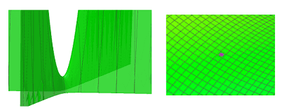
One final, however crucial word: our manifold right here, the saddle, is given by ##M={(x,y,x^2-y^2),|,x,yin mathbb{R}}.## This implies we have now two unbiased parameters, ##x## and ##y,## so ##dim M=2,## a floor. And though we have now embedded it in our three-dimensional area, we won’t care about this embedding, solely concerning the factors on ##M.## The one motive for an embedding is, that we will have fancy photos. Folks on earth don’t acknowledge its curvature except they take a look at the horizon at sea, massive grass savannas, or from outer area.
Physics
Earlier than we hearken to the differential geometer who will inform us one thing about sections and assist clarify the algebraist, allow us to hear what the physicist has to say. Abruptly we discover ourselves in a well-known state of affairs.
The affine area is solely ##{p}+V=T_pM,## the tangent area on the level ##p## of the manifold ##M## outlined by the saddle perform ##z=x^2-y^2.## The metric tensor assigns a bilinear kind to ##T_pM.## So, relying on the place we’re, we have now size, distance, and angle. However physics is all about measurement. How a lot differs one thing if one thing else occurs? In scientific this implies: We want coordinates! And since we already understood the Riemannian manifold ##M,## they are going to be native coordinates; solely legitimate on ##T_pM## and permitting us an inexpensive measurement: symmetric, bilinear (distribution legal guidelines), and non-degenerate (to permit relativity idea) slightly than constructive definiteness.
We have now seen that all of it relies upon (easily) on the placement ##p,## which isn’t any shock since differentiation is an area course of. However we will patch all native views to an atlas. This is the reason we communicate of fields as an alternative of areas. A area is an object obtained by gathering all factors ##pin M.## Subsequently we have now a metric tensor area, and a tangent vector area. It’s normally merely known as a vector area, whereas the vector area of tangents is known as tangent area.
start{align*}
d_p(vec{x}_1,vec{x}_2)=sqrt{g_p(vec{x}_1-vec{x}_2,vec{x}_1-vec{x}_2)}&quadtext{ metric}
g_p(vec{x}_1,vec{x}_2)=D_pvec{x}_1otimes D_pvec{x}_2&quadtext{ metric tensor}
g=bigsqcup_{pin M}g_p=bigcup_{pin M}{p}occasions g_p&quadtext{ metric tensor area}
T_pM&quadtext{ tangent (vector) area}
TM=bigsqcup_{pin M}T_pM=bigcup_{pin M}{p}occasions T_pM&quadtext{ (tangent) vector area}
finish{align*}
Coordinates
Let’s take into account our saddle ##M={(x,y,x^2-y^2):x,yin mathbb{R}}.## A tangent is the rate vector of a curve ##gamma :[0,1]rightarrow M .## We take into account ##gamma^1(t)=(t,p_y,t^2-p_y^2)## and ##gamma^2(t)=(p_x,t,p_x^2-t^2)## via a degree ##p=(p_x,p_y,p_z)in M## and get the tangents ##dotgamma^1(t)=(1,0,2t)## and ##dotgamma^2(t)=(0,1,-2t).## They correspond to the vectors fields ##X_1(p)=D_p(x)=(1,0,2p_x)## and ##X_2(p)=D_p(y)=(0,1,-2p_y).##
By way of degree units, we have now ##f(x,y)=x^2-y^2## and ##(p_x,p_y)in f^{-1}(p_x^2-p_y^2).## Then ##nabla f(p)=(2p_x,-2p_y).## Let additional be ##x,y:[-1,1]rightarrow f^{-1}(p_x^2-p_y^2)## outlined by ##x(t)=(t+p_x,sqrt{(t+p_x)^2-(p_x^2-p_y^2)}),x(0)=(p_x,p_y)## and ##y(t)=(sqrt{(t+p_y)^2+(p_x^2-p_y^2)},t+p_y),y(0)=(p_x,p_y).##
Then
start{align*}
nabla(f(x(0)))cdot dot x(0)&=(2p_x,-2p_y)cdot (1,p_x/p_y)=0
nabla(f(x(0)))cdot dot y(0)&=(2p_x,-2p_y)cdot (p_y/p_x,1)=0
finish{align*}
and the tangent area to the extent set in ##mathbb{R}^2## is ##left{nabla f(p)proper}^perp = operatorname{lin}_mathbb{R}left{(p_y,p_x)proper}##. Thus ##(p_y,p_x,0)=p_yX_1(p)+p_xX_2(p)## is one tangent vector to ##M## at ##p## within the ##z##-plane.
The tangent area with origin in ##p=(2,1,3)## is
$$
T_pM=
operatorname{lin}_mathbb{R}left{X_1(p)=left.dfrac{partial }{partial p_x}proper|_p,X_2(p)=left.dfrac{partial }{partial p_y}proper|_pright}=operatorname{lin_mathbb{R}}left{start{pmatrix}1�4end{pmatrix},start{pmatrix}01-2end{pmatrix} proper}
$$
and the vector area is
$$
TM = bigsqcup_{pin M}operatorname{lin}_mathbb{R}left{X_1=dfrac{partial }{partial p_x},X_2=dfrac{partial }{partial p_y}proper}=bigsqcup_{pin M}operatorname{lin}_mathbb{R}left{start{pmatrix}1�2p_xend{pmatrix},start{pmatrix}01-2p_yend{pmatrix} proper}.
$$
Nevertheless, we don’t wish to hassle with the embedding in ##mathbb{R}^3.## The entire thought about manifolds is, that they don’t require an embedding. There isn’t any Euclidean area across the universe, solely the universe itself. Nicely, we begin a bit smaller and see what the saddle will inform us. However who is aware of, perhaps the universe is a saddle, say a hyperbolic paraboloid. The metric tensor wants vectors as inputs. Our vectors are the tangent vectors ##{X_1(p),X_2(p)}## which kind a foundation for ##V=T_pM.## The affine area ##A## we have now spoken about within the algebra part is solely ##A={p}+T_pM.## These areas are all two-dimensional, so ##g_p## can have 4 parts. To be able to illustrate the dependency on location, we outline in keeping with the body ##mathbf{f}={X_1(p),X_2(p)}##
start{align*}
g_p&triangleq G[mathbf{f}]=g_{ij}[mathbf{f}]=start{pmatrix}
cosh^2 p_x +sinh^2 p_y &0�&(1+4p_x^2+4p_y^2)^{-1}
finish{pmatrix}.
finish{align*}
If we alter the coordinates in ##T_pM## by
##
U_k=(A_{ij})cdot X_k=sum_{l}a_{lk}X_l={a^l}_kX_l
##
then (altering the body)
start{align*}
g(U_i,U_j)&= g({a^ok}_i X_k,{a^l}_jX_l)={a^ok}_i{a^l}_jg(X_k,X_l)
&={a^ok}_i{a^l}_jg_{kl}[mathbf{f}]=sum_{ok,l}(A_{ki})g_{kl}(A_{lj})[mathbf{f}]=left(A^tau cdot G[mathbf{f}]cdot Aright)_{ij}
finish{align*}
and ##G[Amathbf{f}]=A^tau G[mathbf{f}]A,## i.e. the metric tensor, or slightly its coordinate illustration, is known as covariant in physics since its parts remodel like the idea underneath a change of coordinates in every index of the body.
If we alter the coordinate features ##p_x,p_y:Mrightarrow mathbb{R}## to ##q_x,q_y:Mrightarrow mathbb{R}## then
$$
dfrac{partial }{partial q_x}=dfrac{partial p_x}{partial q_x}dfrac{partial }{partial p_x}+dfrac{partial p_y}{partial q_x}dfrac{partial }{partial p_y}; , ;dfrac{partial }{partial q_y}=dfrac{partial p_x}{partial q_y}dfrac{partial }{partial p_x}+dfrac{partial p_y}{partial q_y}dfrac{partial }{partial p_y}
$$
and with the Jacobi matrix ##Dq(p)##
start{align*}
g_{q(p)}&=gleft(dfrac{partial }{partial q_x},dfrac{partial }{partial q_y}proper)=gleft(dfrac{partial p_x}{partial q_x}dfrac{partial }{partial p_x}+dfrac{partial p_y}{partial q_x}dfrac{partial }{partial p_y}, , ,dfrac{partial p_x}{partial q_y}dfrac{partial }{partial p_x}+dfrac{partial p_y}{partial q_y}dfrac{partial }{partial p_y}proper)
finish{align*}
$$
g_{q(p)}=left(left(Dq(p)proper)^{-1}proper)^tau g(p)left(Dq(p)proper)^{-1}
$$
The tangent vectors in our instance are already orthogonal and each diagonal entries are all over the place constructive. ##g_p## has subsequently the signature ##(+,+)## and is a Riemannian metric.
What’s a size in keeping with a metric tensor? The road aspect will be regarded as a line phase related to an infinitesimal displacement vector
$$
ds^2=sum_{i,j}g_{ij}dx_idx_j=g_{ij}dx^idx^j=g_{ij}dfrac{dx^i}{dt}dfrac{dx^j}{dt}dt^2 =g[mathbf{f}]
$$
because it defines the arclength by
$$
s=int_a^b sqrt=int_a^bsqrt{left|g_{ij}(gamma(t))left(dfrac{d}{dt}x^i circ gamma(t)proper)left(dfrac{d}{dt}x^j circ gamma(t)proper)proper|},dt.
$$
The road aspect utterly defines the metric tensor since we thought-about arbitrary curves. That’s the reason it’s typically used as a characterization of the metric tensor slightly than the precise tensor product. In our instance we have now (with ##X_1=D_p(x)=dp_x## and ##X_2=D_p(y)=dp_y##)
$$
ds^2=g=(cosh^2 p_x +sinh^2 p_y ),dp_x^2+(1+4p_x^2+4p_y^2)^{-1},dp_y^2
$$
The notation of the coordinate features as ##p_x,p_y## are supposed to exhibit that we’re contemplating actual valued features ##Mto mathbb{R}.## The same old notation is
$$
ds^2=g=(cosh^2 x +sinh^2 y ),dx^2+(1+4x^2+4y^2)^{-1},dy^2.
$$
The metric tensor at ##(0,0,0)## is given as ##g(0,0,0)=ds^2=dx^2+dy^2## and subsequently the Euclidean metric. The angle between the 2 foundation vectors is ##cossphericalangleleft( X_1(0,0,0),X_2(0,0,0)proper)=0,## i.e. the idea vectors are orthogonal. At ##p=(2,1,3)## we have now a special metric however nonetheless an orthogonal foundation since ##g(2,1,3)((1,0),(0,1))=0## because of the truth that ##g[mathbf{f}]## is diagonal and ##[mathbf{f}]## an orthogonal body. However the lengths of the idea vectors are now not ##1.##
start{align*}
X_1(2,1,3)&=|(1,0)|_{(2,1,3)}=sqrt{cosh^2(2)+sinh^2(1)} approx 3.94
X_2(2,1,3)&=|(0,1)|_{(2,1,3)}= sqrt{1/21}approx 0.22
finish{align*}
Differential Geometry
The differential geometer and the physicist share the toolbox, however not essentially the angle. The primary distinction is perhaps the diploma of abstraction. Emmy Noether spoke of unbiased variables ##p_x,p_y##, dependent features ##q_x(p_x,p_y),q_y(p_x,p_y),## and the applying of a bunch of transformations. Fashionable differential geometers communicate of sections and principal fiber bundles, or Euler-Lagrange equations and differential operators. Emmy Noether’s authentic paper [9] is to some lengthen simpler to know than the trendy remedy of her well-known theorem, cp. [11].
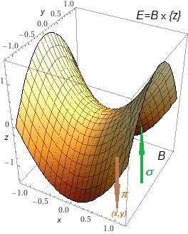
The graph of the perform ##f:Blongrightarrow {z}## is ##{(x,y,x^2-y^2)}=B occasions {z}=Econg mathbb{R}^3.## ##B## is known as the bottom area, right here the ##(x,y)##-plane, and ##E## the entire area, right here your complete ##mathbb{R}^3.## We have now a pure projection ##pi:Elongrightarrow B, , ,(x,y,z)mapsto (x,y).## Any easy perform ##sigma :Blongrightarrow E## such that ##pi(sigma (x,y))=(x,y)## is known as a piece, and the set of all sections is denoted by ##Gamma(E).## However what does this should do with differentiation and the saddle? We already launched the (tangent) vector area, which can be known as tangent bundle or simply vector bundle.
$$
E=TM=bigsqcup_{pin M}T_pM=bigcup_{pin M}{p}occasions T_pM
$$
the place the tangent areas are the bottom area isomorphic to ##mathbb{R}^2## and ##sigma(p_x,p_y)=(p_x,p_y,p_x^2-p_y^2)## are the sections. The preimage ##pi^{-1}(p_x,p_y)={p}occasions T_pM## is known as fiber (over ##p=(p_x,p_y)##). Bundle as a result of we take into account units of factors, i.e. bundles (units) of fibers. That is additionally the explanation why we use the notation with ##sqcup_p.## To be exact, we must always have launched the cotangent bundle as an alternative as a result of our metric tensor is outlined as
$$
Gamma((TMotimes TM)^*ni g , , ,g_p in T_p^*Motimes T_p^*M = (T_pMotimes T_pM)^*
$$
If we have now a bunch working on the fibers then we communicate of principal bundles. Emmy Noether’s group of easy transformations is the group that operates on a precept bundle, and its smoothness qualifies it as a Lie group.
Levi-Civita Connection
A connection is a directional spinoff by way of vector fields comparable with the gradient. The Levi-Civita connection is torsion-free and preserves the Riemannian metric tensor. It’s also known as the covariant spinoff alongside a curve
$$
nabla_{dotgamma(0)} sigma(p) =(sigma circ gamma )'(0)=lim_{t to 0}dfrac{sigma (gamma (t))-sigma (p)}{t},
$$
or Riemannian connection. Its existence and uniqueness are generally known as the elemental theorem of Riemmanian geometry. An (affine) connection is formally outlined as a bilinear map
$$
nabla, : ,Gamma(TM)timesGamma(TM) longrightarrow Gamma(TM), , ,(X,Y)longmapsto nabla_XY
$$
that’s ##C^infty (M)##-linear within the first argument, ##mathbb{R}##-linear within the second, and obeys the Leibniz rule ##nabla_X(hsigma )=X(h)cdot sigma +hcdot nabla_X(sigma).## The Levi-Civita connection is an affine connection that’s torsion-free, i.e. ##nabla_XY-nabla_YX=[X,Y]## with the Lie bracket of vector fields, and preserves the metric, i.e.
$$
Z(g(X,Y))=g(nabla_Z X,Y)+g(X,nabla_Z Y))textual content{ or quick }nabla_Z g(X,Y)=0.
$$
The distinction to a Lie spinoff is, {that a} Lie spinoff is ##mathbb{R}##-linear however doesn’t should be ##C^infty (M)##-linear. We additionally point out the Koszul method
start{align*}
g(nabla_{X}Y,Z)&={tfrac{1}{2}}{Massive {}X{bigl (}g(Y,Z){bigr )}+Y{bigl (}g(Z,X){bigr )}-Z{bigl (}g(X,Y){bigr )}&phantom{=}+g([X,Y],Z)-g([Y,Z],X)-g([X,Z],Y){Massive }}.
finish{align*}
If we write with Christoffel symbols ##Gamma_{ij}^ok##
$$
nabla_jpartial_k =Gamma_{jk}^lpartial_l
$$
then $$
nabla_XY=X^jleft(partial_j(Y^l)+Y^kGamma_{jk}^lpartial_lright) $$
and ##nabla## is suitable with the metric if and provided that
$$partial_{i}{bigl (}g(partial_{j},partial_{ok}){bigr )}=g(nabla_{i}partial_{j},partial_{ok})+g(partial_{j},nabla_{i}partial_{ok})=g(Gamma_{ij}^{l}partial_{l},partial_{ok})+g(partial_{j},Gamma_{ik}^{l}partial_{l}),$$
i.e. ##partial_{i}g_{jk}=Gamma_{ij}^{l}g_{lk}+Gamma_{ik}^{l}g_{jl}.## It’s torsion-free if
$$
nabla_{i}partial_{j}-nabla_{j}partial_{i}=(Gamma_{jk}^{l}-Gamma_{kj}^{l})partial_{l}=[partial_{i},partial_{j}]=0,$$
i.e. ##Gamma_{jk}^{l}=Gamma_{kj}^{l}.## We will examine by direct calculation that
$$Gamma_{jk}^{l}={tfrac{1}{2}}g^{lr}left(partial_{ok}g_{rj}+partial_{j}g_{rk}-partial_{r}g_{jk}proper)$$
the place ##g^{lr}## stands for the inverse metric ##(g_{lr})^{-1}.##
Let ##gamma(t):[-1,1]longrightarrow M## be a easy curve on the manifold ##M.## A piece ##sigma in Gamma(TM)## alongside ##gamma ## is known as parallel in keeping with ##nabla## if
$$nabla_{dotgamma(t)}sigma (gamma(t))=0 textual content{ for all } t.$$
This implies in case of tangent vectors of tangent bundles of a manifold that each one tangent vectors are fixed with respect to an infinitesimal displacement from ##gamma(t)## within the route of ##dotgamma(t).## A vector area is known as parallel whether it is parallel with respect to each curve within the manifold. Let ##t_0,t_1in [-1,1].## Then there’s a distinctive parallel vector area ##Y:Mrightarrow T_{gamma(t)}M## alongside ##gamma ## for each ##X_pin T_{gamma(t_0)}M## such that ##X_p=Y_{gamma (t_0)}.## The perform
$$ P_{gamma(t_{0}),gamma(t_{1})}colon T_{gamma(t_{0})}Mto T_{gamma(t_{1})}M,quad X_pmapsto Y_{gamma(t_{1})} $$
is known as parallel transport. The existence and uniqueness comply with from the worldwide model of the Picard-Lindelöf theorem for odd linear differential equation methods. We have now completely different internal merchandise at ##t_0## and ##t_1,## and thus completely different metrics. A parallel transport determines what occurs alongside a path from one tangent area to the opposite.
We have now commuting two-dimensional vector fields in our instance of the two-dimensional saddle ##M## as a result of the partial derivatives commute. This implies we have now ##nabla_{X_1}X_2=nabla_{X_2}X_1.## Moreover, the metric is diagonal, i.e. solely stretches and compressions alongside the coordinate features. Let
$$
%gamma: [-1,1] rightarrow M, , ,gamma(t)=(2t+1,t+1/2,3(t+1/2)^2)
gamma : [-1,1] rightarrow M, , ,gamma(t)=(2t+1,t+1/2)
$$
with ##p=gamma(-1/2)=(0,0)## and ##q=gamma(1/2)=(2,1).## We have to resolve
$$
nabla_{(2,1)}sigma(2t+1,t+1/2)= lim_{t’ to t}dfrac{sigma(2t’+1,t’+1/2)-sigma(2t+1,t+1/2)}{t’} =0
$$
which is clearly true for a (easy) part of ##Gamma(TM).## The parallel transport is solely given by protecting the parts of the vector fields. ##X_p=alpha X_1(p)+beta X_2(p)## maps to ##Y_{q}=alpha X_1(q)+beta X_2(q).## This implies within the three dimensions of the embedding
$$
start{pmatrix}alpha beta � finish{pmatrix}longmapsto start{pmatrix}2t+1t+1/23(t+1/2)^2end{pmatrix}+start{pmatrix}alpha beta 4alpha t +2alpha -2beta t-beta finish{pmatrix}.
$$
[ad_2]