The Artwork of Integration | Physics Boards
[ad_1]
Summary
My college trainer used to say
“Everyone can differentiate, but it surely takes an artist to combine.”
The mathematical cause behind this phrase is, that differentiation is the calculation of a restrict
$$
f'(x)=lim_{vto 0} g(v)
$$
for which now we have many guidelines and theorems at hand. And if nothing else helps, we nonetheless can draw ##f(x)## and a tangent line. Geometric integration, nevertheless, is restricted to rudimentary examples and even easy integrals such because the finite quantity of Gabriel’s horn with its infinite floor are laborious to visualise. A gallon of paint is not going to match inside but is inadequate to color its floor?!

Whereas the integrals of Gabriel’s horn
$$
textual content{quantity }=piint_1^infty dfrac{1}{x^2},dx; textual content{ and } ;textual content{floor }=2piint_1^infty dfrac{1}{x},sqrt{1+dfrac{1}{x^4}},dx
$$
can presumably be solved by Riemann sums and thus with restrict calculations, too, a perform like
$$
dfrac{log x}{a+1-x}-dfrac{log x}{a+x}quad (ain mathbb{C}backslash[-1,0])
$$
which is straightforward to distinguish
$$
dfrac{d}{dx}left(dfrac{log x}{a+1-x}-dfrac{log x}{a+x}proper)=
dfrac{1}{x(a+1-x)}+dfrac{log x}{(a+1-x)^2}-dfrac{1}{x(a+x)}-dfrac{log x}{(a+x)^2}
$$
can’t be built-in straightforwardly. Earlier than I symbolize the most important strategies of integration which would be the content material of this text, allow us to have a look at just a little piece of artwork.
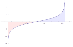
We wish to discover the anti-derivative
$$
int_0^1 left(dfrac{log x}{a+1-x}-dfrac{log x}{a+x}proper),dx
$$
Outline ##F, : ,]0,1]longrightarrow mathbb{C}## by ##F(x):=dfrac{xlog x}{a+x}-log(a+x).##
Then
start{align*}
F'(x)&=dfrac{(a+x)(1+log x)-xlog x}{(a+x)^2}-dfrac{1}{a+x}=dfrac{alog x}{(a+x)^2}
finish{align*}
and
$$
aint_0^1 dfrac{log x}{(a+x)^2},dx=F(1)-F(0^+)=-log(a+1)-(-log a)=log a -log (a+1).
$$
Subsequent, we outline ##G, : ,]0,1]longrightarrow mathbb{C}## by ##G(x):=dfrac{xlog x}{a+1-x}+log(a+1-x).##
Then
start{align*}
G'(x)&=dfrac{(a+1-x)(1+log x)+xlog x}{(a+1-x)^2}-dfrac{1}{a+1-x}=dfrac{(a+1)log x}{(a+1-x)^2}
finish{align*}
and
$$
(a+1)int_0^1dfrac{log x}{(a+1-x)^2},dx=G(1)-G(0^+)=log a-log(a+1).
$$
Lastly, these integrals can be utilized to calculate
start{align*}
I(a)&=int_0^1 left(dfrac{log x}{a+1-x}-dfrac{log x}{a+x}proper),dx =int_0^1 int left(dfrac{log x}{(a+x)^2}-dfrac{log x}{(a+1-x)^2}proper),da,dx
&=int left(left(dfrac{1}{a}-dfrac{1}{a+1}proper)cdotleft(log a -log (a+1)proper)proper),da =dfrac{1}{2}left(log a -log (a+1)proper)^2+C.
finish{align*}
From ##displaystyle{lim_{a to infty}I(a)=0}## we get ##C=0## and so
$$
int_0^1 left(dfrac{log x}{a+1-x}-dfrac{log x}{a+x}proper),dx=dfrac{1}{2}left(log dfrac{a}{a+1}proper)^2.
$$
The Basic Theorem of Calculus
If ##f:[a,b]rightarrow mathbb{R}## is a real-valued steady perform, then there exists a differentiable perform, the anti-derivative, ##F:[a,b]rightarrow mathbb{R}## such that
$$
F(x)=int_c^tf(t),dt textual content{ for }cin [a,b]textual content{ and }F'(x)=f(x)
$$
Furthermore $$int_a^b f(x),dx = left[F(x)right]_a^b=F(b)-F(a)$$
Imply Worth Theorem of Integration
$$
int_a^b f(x)g(x),dx =f(xi) int_a^b g(x),dx
$$
for a steady perform ##f:[a,b]rightarrow mathbb{R}## and an integrable perform ##g## that has no signal adjustments, i.e. ##g(x) geq 0## or ##g(x)leq 0## on ##[a,b];,,xiin [a,b].##
$$
int_a^b f(x)g(x),dx = f(a)int_a^xi g(x),dx +f(b) int_xi^b g(x),dx
$$
if ##f(x)## is monotone, ##g(x)## steady.
These theorems are extra essential for estimations of integral values than truly computing their worth.
Fubini’s Theorem
$$
int_{Xtimes Y}f(x,y),d(x,y)=int_Y int_Xf(x,y),dx,dy=int_Xint_Y f(x,y),dy,dx
$$
for steady features ##f, : ,Xtimes Y rightarrow mathbb{R}.## It is likely one of the most used theorems at any time when an space or a quantity must be computed. Nevertheless, we want steady features! An instance the place the concept can’t be utilized:
$$
underbrace{int_0^1int_0^1 dfrac{x-y}{(x+y)^3},dx,dy}_{=-1/2} =int_0^1int_0^1 dfrac{y-x}{(y+x)^3},dy,dx=-underbrace{int_0^1int_0^1dfrac{x-y}{(x+y)^3},dy,dx}_{=+1/2}
$$
Partial Fraction Decomposition
We nearly used partial fraction decomposition within the earlier instance when the issue ##dfrac{1}{a}-dfrac{1}{a+1}=dfrac{1}{a(a+1)}## within the integrand occurred. Equations like this are meant by partial fraction decomposition. Whereas ##dfrac{1}{a(a+1)}## seems to be troublesome to combine, the integrals of ##dfrac{1}{a}## and ##dfrac{1}{a+1}## are easy logarithms. Assume now we have polynomials ##p_k(x)## and an integrand
$$
q_0(x)prod_{okay=1}^m p_k^{-1}(x)=dfrac{q_0(x)}{prod_{okay=1}^m p_k(x)}stackrel{!}{=}sum_{okay=1}^m dfrac{q_k(x)}{p_k(x)}=sum_{okay=1}^m dfrac{q_k(x)prod_{ineq okay}p_i(x)}{prod_{okay=1}^m p_k(x)}.
$$
Then all we want are appropriate polynomials ##q_k(x)## such that
$$
q_0(x)=sum_{okay=1}^m q_k(x)prod_{ineq okay}p_i(x)
$$
holds and every of the ##m## many phrases is straightforward to combine. The bounds of this method are apparent: the levels of the polynomials on the precise needs to be small. Partial fraction decomposition is certainly often used if the levels of ##q_k(x)## are quadratic at most, the much less the higher.
Instance: Combine ##displaystyle{int_2^{10} dfrac{x^2-x+4}{x^4-1},dx.}## This implies now we have to unravel
$$
x^2-x+4=q_1(x)underbrace{(x+1)(x-1)}_{x^2-1}+q_2(x)underbrace{(x^2+1)(x+1)}_{x^3+x^2+x+1}+q_3(x)underbrace{(x^2+1)(x-1)}_{x^3-x^2+x-1}
$$
Our unknowns are the polynomials ##q_k(x).## We set ##q_k=a_kx+b_k## and get by evaluating the coefficients
start{align*}
x^4, &: ,0= a_2+a_3
x^3, &: ,0= a_1+a_2-a_3+b_2+b_3
x^2, &: ,1= a_2+a_3+b_1+b_2-b_3
x^1, &: ,-1= -a_1+a_2-a_3+b_2+b_3
x^0, &: ,4= -b_1+b_2-b_3
finish{align*}
One answer is due to this fact ##q_1(x)=dfrac{x-3}{2}, , ,q_2(x)=x, , ,q_3(x)=-dfrac{2x+5}{2}## and
start{align*}
int_2^{10} &dfrac{x^2-x+4}{x^4-1},dx =dfrac{1}{2}int_2^{10} dfrac{x}{x^2+1},dx – dfrac{3}{2}int_2^{10} dfrac{1}{x^2+1},dx
&phantom{=}+int_2^{10}dfrac{x}{x-1},dx -int_2^{10}dfrac{x}{x+1},dx-dfrac{5}{2}int_2^{10}dfrac{1}{x+1},dx
&=dfrac{1}{4}left[phantom{dfrac{}{}}log(x^2+1)right]_2^{10}-dfrac{3}{2}left[phantom{dfrac{}{}}operatorname{arc tan}(x)right]_2^{10}
&phantom{=}+left[phantom{dfrac{}{}}x+log( x-1)right]_2^{10}-left[phantom{dfrac{}{}}x-log(x+1)right]_2^{10}-dfrac{5}{2}left[phantom{dfrac{}{}}log(x+1)right]_2^{10}
&=-dfrac{3}{2}(operatorname{arctan}(10)-operatorname{arctan}(2))+dfrac{1}{4}logleft(dfrac{101cdot 9^4cdot 3^6}{5cdot 11^6}proper)approx 0,45375ldots
finish{align*}
Integration by Elements – The Leibniz Rule
Integration by elements is one other means to take a look at the Leibniz rule.
start{align*}
(u(x)cdot v(x))’&=u(x)’cdot v(x)+u(x)cdot v(x)’
int (u(x)cdot v(x))’, dx&=int u(x)’cdot v(x),dx+int u(x)cdot v(x)’,dx
int_a^b u(x)’cdot v(x),dx &=left[u(x)v(x)right]_a^b -int_a^b u(x)cdot v(x)’,dx
finish{align*}
It’s a chance to shift the issue of integration of a product from one issue to the opposite, e.g.
start{align*}
int xlog x,dx&=dfrac{x^2}{2}log x-int dfrac{x^2}{2}cdot dfrac{1}{x},dx=dfrac{x^2}{4}left(-1+2log x proper)
finish{align*}
Integration by elements is particularly helpful for trigonometric features the place we will use the periodicity of sine and cosine below differentiation, e.g.
start{align*}
int sin xcos x,dx&=-cos^2 x-int cos xsin x,dx
int sin xcos x,dx&=-dfrac{1}{2}cos^2 x=dfrac{1}{2}(-1+sin^2 x)
int cos^2 x ,dx&=x-int sin^2x,dx=x+cos xsin x-int cos^2x,dx
&=dfrac{1}{2}(x+cos xsin x)
finish{align*}
part{Integration by Discount Formulation}
Integration by elements typically gives recursions that result in so-called discount formulation since they successively lower a amount, often an exponent. Which means an integral
$$
I_n=int f(n,x),dx
$$
might be expressed as a linear mixture of integrals ##I_k## with ##okay<n.## E.g.
start{align*}
underbrace{int x^n e^{alpha x},dx}_{=I_n}&= left[x^{n}alpha^{-1}e^{alpha x}right]-nalpha^{-1}underbrace{int x^{n-1} e^{alpha x},dx}_{=I_{n-1}}
finish{align*}
or
start{align*}
int cos^nx,dx&=left[sin xcos^{n-1}xright]+(n-1)int sin^2 xcos^{n-2}x,dx
&=left[sin xcos^{n-1}xright]+(n-1)int cos^{n-2}x,dx-(n-1)int cos^n,dx
finish{align*}
which ends up in the discount components
$$
int cos^nx,dx=dfrac{1}{n}left[sin xcos^{n-1}xright]+dfrac{n-1}{n}intcos^{n-2}x,dx
$$
Discount formulation might be difficult, and so they can have multiple pure quantity as parameters, cp.[1]. The discount components for the sine is
$$
int sin^nx,dx=-dfrac{1}{n}left[sin^{n-1} xcos xright]+dfrac{n-1}{n}intsin^{n-2}x,dx
$$
Lobachevski’s Formulation
Let ##f(x)## be a real-valued steady perform that’s ##pi## periodic, i.e. ##f(x+pi)=f(x)=f(pi-x)## for all ##xgeq 0,## e.g. ##f(x)equiv 1.## Then
start{align*}
int_{0}^{infty }{dfrac{sin^{2}x}{x^{2}}}f(x),dx &=int_{0}^{infty }{dfrac{sin x}{x}}f(x),dx
=int_{0}^{pi /2}f(x),dx[6pt]
int_{0}^{infty }{dfrac{sin^{4}x}{x^{4}}}f(x),dx&
=int_{0}^{pi /2}f(t),dt-{dfrac{2}{3}}int_{0}^{pi /2}sin^{2}tf(t),dt
finish{align*}
This ends in the formulation
$$
int_{0}^{infty }{dfrac{sin x}{x}},dx=int_{0}^{infty }{dfrac{sin^{2}x}{x^{2}}},dx={dfrac{pi }{2}}
; textual content{ and } ; int_{0}^{infty }{dfrac{sin^{4}x}{x^{4}}},dx={dfrac{pi }{3}}.
$$
Substitutions
The Chain Rule
Substitutions are most likely probably the most utilized method. Barely an integral that doesn’t use it, or how I prefer to put it:
Do away with what disturbs probably the most!
Substitution is technically a metamorphosis of the mixing variable, a change of coordinates, the chain rule!
start{align*}
int_a^b f(g(x)),dx stackrel{y=g(x)}{=}int_{g(a)}^{g(b)} f(y)cdot left(dfrac{dg(x)}{dx}proper)^{-1},dy
finish{align*}
Observe that the mixing limits change, too! After all, not any coordinate transformation is useful, and what seems to be as if we difficult issues can truly simplify the integral. We will take away the disturbing perform ##g(x)## at any time when both ##g'(x)## or ##f(x)/g'(x)## are particularly easy, e.g.
start{align*}
int_0^2 xcos (x^2+1),dxstackrel{;y=x^2+1}{=}&int_1^5 xcos ydfrac{dy}{2x}=dfrac{1}{2}int_1^5cos y,dy =dfrac{1}{2}(sin (5)-sin (1))
int_0^1sqrt{1-x^2},dxstackrel{y=arcsin x}{=}&int_{0}^{pi/2}cos^2 y,dy=left[dfrac{1}{2}(x+cos x sin x)right]_0^{pi/2}=dfrac{pi}{4}
finish{align*}
start{align*}
int_{-infty}^{infty} f(x),dfrac{tan x}{x},dx =& sum_{kin mathbb{Z}} int_{(k-1/2) pi }^{(okay+1/2)pi}f(x),dfrac{tan x}{x},dx
stackrel{y=x-kpi}{=} sum_{kin mathbb{Z}} int_{-pi /2 }^{pi /2 } f(y) ,dfrac{tan y}{y+kpi},dy
=&int_{-pi /2 }^{pi /2 }f(y)underbrace{sum_{kin mathbb{Z}} dfrac{1}{y+kpi}}_{=cot y} ,tan y, dy
stackrel{z=y+pi /2}{=} int_{0}^{pi }f(z),dz
finish{align*}
Weierstraß Substitution
The Weierstraß substitution or tangent half-angle substitution is a way that transforms trigonometric features into rational polynomial features. We begin with
$$
tanleft(dfrac{x}{2}proper) = t
$$
and get
$$
sin x=dfrac{2t}{1+t^2}; , ;cos x=dfrac{1-t^2}{1+t^2}; , ;
dx=dfrac{2}{1+t^2},dt.
$$
These substitutions are particularly helpful in spherical geometry. The next examples could illustrate the precept.
start{align*}
int_0^{2pi}dfrac{dx}{2+cos x}&=int_{-infty }^infty dfrac{2}{3+t^2},dtstackrel{t=usqrt{3}}{=}dfrac{2}{sqrt{3}}int_{-infty }^infty dfrac{1}{1+u^2},du=dfrac{2pi}{sqrt{3}}
finish{align*}
start{align*}
int_0^{pi} dfrac{sin(varphi)}{3cos^2(varphi)+2cos(varphi)+3},dvarphi &= int_0^infty dfrac{t}{t^4+2}~dt stackrel{u=frac{1}{2}t^2}{=}
= frac{1}{2sqrt{2}}int_0^infty dfrac{du}{1+u^2}
&= frac{1}{2sqrt{2}}left[phantom{dfrac{}{}}operatorname{arctan} u;right]_0^infty=frac{pi}{4sqrt{2}}
finish{align*}
Euler Substitutions
Euler substitutions are a way to deal with integrands which are rational expressions of sq. roots of a quadratic polynomial
$$
int Rleft(x,sqrt{ax^2+bx+c},proper),dx.
$$
Allow us to first have a look at an instance. With a purpose to combine
$$int_1^5 dfrac{1}{sqrt{x^2+3x-4}},dx$$
we have a look at the zeros of the quadratic polynomial ##sqrt{x^2+3x-4}=sqrt{(x+4)(x-1)}.## We get from the substitution ##sqrt{(x+4)(x-1)}=(x+4)t##
$$x=dfrac{1+4t^2}{1-t^2}; , ;sqrt{x^2+3x-4}=dfrac{5t}{1-t^2}; , ;dx = dfrac{10t}{(1-t^2)^2},dt$$
start{align*}
int_1^5 frac{dx}{sqrt{x^2+3x-4}}&=int_{0}^{2/3}dfrac{2}{1-t^2},dt=int_{0}^{2/3}dfrac{1}{1+t},dt+int_{0}^{2/3}dfrac{1}{1-t},dt[6pt]
&=left[log(1+t)-log(1-t)right]_0^{2/3}=log(5)
finish{align*}
This was the third of Euler’s substitutions. All in all, now we have
- Euler’s First Substitution.
$$
sqrt{ax^2+bx+c}=pm sqrt{a}cdot x+t, , ,x=dfrac{c-t^2}{pm 2tsqrt{a}-b}; , ;a>0
$$ - Euler’s Second Substitution.
$$
sqrt{ax^2+bx+c}=xtpm sqrt{c}, , ,x=dfrac{pm 2tsqrt{c}-b}{a-t^2}; , ;c>0
$$ - Euler’s Third Substitution.
$$
sqrt{ax^2+bx+c}=sqrt{a(x-alpha)(x-beta)}=(x-alpha)t, , ,x=dfrac{abeta-alpha t^2}{a-t^2}
$$
Transformation Theorem
The chain rule works equally for features in multiple variable. Let ##Usubseteq mathbb{R}^n## be an open set and ##varphi , : ,Urightarrow mathbb{R}^n## a diffeomorphism, and ##f## an actual valued perform outlined on ##varphi(U).## Then
$$
int_{varphi(U)} f(y),dy=int_U f(varphi (x))cdot |det underbrace{(Dvarphi(x) )}_{textual content{Jacobi matrix}}|,dx.
$$
That is particularly attention-grabbing if ##fequiv 1,## in order that the components turns into
$$
operatorname{vol}(varphi(U))=int_U |det (Dvarphi(x))|,dx = |det (Dvarphi(x))|cdotoperatorname{vol}(U),
$$
or in any instances the place the determinant equals one, e.g. for orthogonal transformations ##varphi ,## like rotations. For instance, we calculate the world beneath the Gaussian bell curve.
start{align*}
int_{-infty }^infty dfrac{1}{sigma sqrt{2pi}} e^{-frac{1}{2}left(frac{x-mu}{sigma}proper)^2},dx&stackrel{t=frac{x-mu}{sigma sqrt{2}}}{=}
dfrac{1}{sqrt{pi}} int_{-infty }^infty e^{-t^2},dtstackrel{!}{=}1
finish{align*}
As an alternative of immediately calculating the integral, we are going to present that
$$
left(int_{-infty }^infty e^{-t^2},dtright)^2=int_{-infty }^infty e^{-x^2},dx cdot int_{-infty }^infty e^{-y^2},dy=int_{-infty }^inftyint_{-infty }^infty e^{-x^2-y^2},dx,dy=pi
$$
and make use of the truth that ##f(x,y)=e^{-x^2-y^2}=e^{-r^2}## is rotation-symmetric, i.e. we are going to make use of polar coordinates. Let ##U=mathbb{R}^+instances (0,2pi)## and ##varphi(r,alpha)=(rcos alpha,r sin alpha).##
start{align*}
det start{pmatrix}dfrac{partial varphi_1 }{partial r }&dfrac{partial varphi_1 }{partial alpha }[12pt] dfrac{partial varphi_2 }{partial r }&dfrac{partial varphi_2 }{partial alpha }finish{pmatrix}=det start{pmatrix}cos alpha &-rsin alpha sin alpha &rcos alphaend{pmatrix}=r
finish{align*}
and at last
start{align*}
int_{-infty }^inftyint_{-infty }^infty &e^{-x^2-y^2},dx,dy=int_{varphi(U)}e^{-x^2-y^2},dx,dy
&=int_U e^{-r^2cos^2alpha -r^2sin^2alpha }cdot |det(Dvarphi)(r,alpha)|,dr,dalpha
&=int_0^{2pi}int_0^infty re^{-r^2},dr,dalphastackrel{t=-r^2}{=}int_0^{2pi}dfrac{1}{2}int_{-infty }^0 e^{t},dt ,dalpha=int_0^{2pi}dfrac{1}{2},dalpha =pi
finish{align*}
Translation Invariance
$$
int_{mathbb{R}^n} f(x),dx = int_{mathbb{R}^n} f(x-c),dx
$$
is nearly self-explaining since we combine over the whole area. Nevertheless, there are much less apparent instances
$$
int_{-infty}^{infty} fleft(x-dfrac{b}{x}proper),dx=int_{-infty}^{infty}f(x),dx, textual content{ for any } ,b>0
$$
textbf{Proof:} From
$$int_{-infty}^{infty}fleft(x-dfrac{b}{x}proper),dx
stackrel{u=-b/x}{=}int_{-infty}^{infty} fleft(u-dfrac{b}{u}proper)dfrac{b}{u^2},du$$
we get
start{align*}
int_{-infty}^{infty} fleft(x-dfrac{b}{x}proper),dx &+int_{-infty}^{infty} fleft(x-dfrac{b}{x}proper),dx=int_{-infty}^{infty} fleft(x-dfrac{b}{x}proper)left(1+dfrac{b}{x^2}proper),dx
&= int_{-infty}^{0} fleft(x-dfrac{b}{x}proper)left(1+dfrac{b}{x^2}proper),dx +int_{0}^{infty} fleft(x-dfrac{b}{x}proper)left(1+dfrac{b}{x^2}proper),dx
&stackrel{v=x-(b/x)}{=} int_{-infty}^{infty} f(v),dv +int_{-infty}^{infty} f(v),dv=2int_{-infty}^{infty} f(v),dv
finish{align*}
which proves the assertion.
Symmetries
Symmetries are the core of arithmetic and physics basically. So it doesn’t shock that they play an important position in integration, too. The precept is a simplification:
$$
int_{-c}^c |x|,dx= 2cdot int_0^c x,dx = c^2
$$
Additive Symmetry
A bit extra subtle instance for additive symmetry is ##displaystyle{int_0^{pi/2}}log (sin(x)),dx.##
We use the symmetry between the sine and cosine features.
start{align*}
int_0^{pi/2}log (sin x),dx&=-int_{pi/2}^0log (cos x),dx=int_0^{pi/2}log (cos x),dx
finish{align*}
start{align*}
2int_0^{pi/2}log (sin x),dx&=int_0^{pi/2}log (sin x),dx+int_0^{pi/2}log (cos x ,dx
&=int_0^{pi/2}log(sin x cos x)=int_0^{pi/2}logleft(dfrac{sin 2x}{2}proper),dx
&stackrel{u=2x}{=}-dfrac{pi}{2}log 2+dfrac{1}{2}int_0^{pi}log(sin u),du
&=-dfrac{pi}{2}log 2+int_0^{pi/2}log(sin u),du
finish{align*}
We thus have ##displaystyle{int_0^{pi/2}log (sin x),dx=-dfrac{pi}{2}log 2.}##
We will in fact calculate symmetric areas. That simplifies the mixing boundaries.

The world of an astroid is enclosed by ##(x,y)=(cos^3 t,sin^3 t)## for ##0leq t leq 2pi.##
$$
4int_0^1 y,dxstackrel{x=cos^3(t)}{=}-12int_{pi/2}^0 sin^4 tcdot cos^2 t ,dt = dfrac{3}{8}pi
$$
Multiplicative Symmetry
A bit much less well-known are presumably the multiplicative symmetries. We nearly bumped into one within the instance within the translation paragraph earlier than it lastly turned out to be an additive symmetry. Let’s illustrate with some examples what we imply, e.g. with a multiplicative asymmetry.
$$
int_0^pilog(1-2alpha cos(x)+alpha^2),dx=2pilog |alpha|; , ;|alpha|geq 1
$$
however how can we all know? We begin with a price ##|alpha|leq 1## and ##0<x<pi.## Then by Gradshteyn, Ryzhik 1.514 [6]
$$
log(1-2alpha cos(x)+alpha^2)= -2sum_{okay=1}^{infty}dfrac{cos(kx)}{okay},alpha^okay
$$
and
##displaystyle{I(alpha)=int_0^pi log (1-2alpha cos(x)+alpha^2),dx = -2sum_{okay=1}^{infty} dfrac{alpha^okay}{okay} int_{0}^{pi} cos(kx),dx =0}.##
This implies for ##|alpha|geq 1##
start{align*}
int_0^pi log (1-2alpha cos(x)+alpha^2),dx &= int_0^pi logleft(alpha^2 left(dfrac{1}{alpha^2}-dfrac{2}{alpha}cos(x)+1right)proper),dx
&=2pi log|alpha| + underbrace{Ileft(dfrac{1}{alpha}proper)}_{=0}= 2pi log|alpha|
finish{align*}
So we used a consequence about ##I(1/a)## to calculate ##I(a).## The subsequent instance makes use of the multiplicative symmetry of the mixing variable
start{align*}
int_{n^{-1}}^{n} fleft(x+dfrac{1}{x}proper),dfrac{log x}{x},dx &stackrel{y=1/x}{=} int_{n}^{n^{-1}}fleft(dfrac{1}{y}+yright),dfrac{log y}{y},dy
&=-int_{n^{-1}}^{n} fleft(x+dfrac{1}{x}proper),dfrac{log x}{x},dx
finish{align*}
which is just doable if the mixing worth is zero. By related arguments
$$
int_{frac{1}{2}}^{3} dfrac{1}{sqrt{x^2+1}},dfrac{log(x)}{sqrt{x}},dx , + , int_{frac{1}{3}}^{2} dfrac{1}{sqrt{x^2+1}},dfrac{log(x)}{sqrt{x}},dx =0
$$
and
$$
int_{pi^{-1}}^pi dfrac{1}{x}sin^2 left( -x-dfrac{1}{x} proper) log x,dx=0
$$
Including an Integral
It’s generally useful to rewrite an integrand with an extra integral, e.g. for ##alphanotin mathbb{Z}##
start{align*}
int_0^infty dfrac{dx}{(1+x)x^alpha} &= int_0^infty x^{-alpha} int_0^infty e^{-(1+x)t},dt,dx=int_0^inftyint_0^infty x^{-alpha} e^{-t}e^{-xt},dt,dx
&stackrel{u=tx}{=}int_0^inftyint_0^infty left(dfrac{u}{t}proper)^{-alpha}e^{-u}e^{-t}t^{-1},du,dx
&=int_0^infty u^{-alpha}e^{-u},du, int_0^infty t^{alpha -1} e^{-t},dt=Gamma (1-alpha) Gamma(alpha)=dfrac{pi}{sin pi alpha}
finish{align*}
or
start{align*}
&int_0^infty frac{x^{m}}{x^{n} + 1}dx = int_0^infty x^{m} int_0^infty e^{-x^n y} e^{-y} ,dy, dx
&stackrel{z=x^ny}{=}dfrac{1}{n} int_0^infty e^{-y} left(frac{1}{y}proper)^frac{m+1}{n} ,dy int_0^infty e^{-z} z^frac{m-n+1}{n} ,dz= dfrac{Gammaleft(dfrac{n-m-1}{n}proper) Gammaleft(dfrac{m+1}{n}proper)}{n}
finish{align*}
The Mass at Infinity
If ##f_k: Xrightarrow mathbb{R}## is a sequence of pointwise absolute convergent, integrable features, then
$$
int_X left(sum_{okay=1}^infty f_k(x)proper),dx=sum_{okay=1}^infty left(int_X f_k(x),dxright)
$$
Instance: The Wallis Collection.
start{align*}
int_0^{pi/2}dfrac{2sin x}{2-sin^2 x},dx&=int_0^{pi/2}dfrac{2sin x}{1+cos x},dx=left[-2arctan(cos x)right]_0^{pi/2}=dfrac{pi}{2}
&=int_0^{pi/2}dfrac{sin x}{1-frac{1}{2}sin^2 x},dx=int_0^{pi/2}sum_{okay=0}^infty 2^{-k}sin^{2k+1}x ,dx
&=sum_{okay=0}^inftyint_0^{pi/2}2^{-k}sin^{2k+1}x ,dx=sum_{okay=0}^inftydfrac{1cdot 2cdot 3cdots okay}{3cdot 5 cdot 7 cdots (2k+1)}
finish{align*}
Absolutely the convergence is essential as we will see within the following instance. Let ##f_k=I_{[k,k+1,]}-I_{[k+1,k+2]}## with the indicator perform ##I_{[k,k+1,]}(x)=1## if ##xin[k,k+1]## and ##I_{[k,k+1,]}(x)=0## in any other case. If we sum up these features, we get a telescope impact. The bump at ##[0,1]## stays untouched whereas the bump (the mass) ##[k+1,k+2]## escapes to infinity: ##displaystyle{sum_{okay=0}^n}f_k=I_{[0,1,]}-I_{[n+1,n+2]}## and ##displaystyle{sum_{okay=1}^infty f_k(x)}=I_{[0,1,]}(x).## Therefore,
$$
1=int_mathbb{R}I_{[0,1,]}(x),dx=int_mathbb{R} left(sum_{okay=1}^infty f_k(x)proper),dxneq sum_{okay=1}^infty left(int_mathbb{R} f_k(x),dxright)=0.
$$
Limits and Integrals
Mass at infinity is strictly an change of a restrict and an integral. So what about limits basically? Even when all features ##f_k## of a convergent sequence are steady or integrable, the identical just isn’t essentially true for the restrict. Have a look at
$$
f_k(x)=start{instances}okay^2x &textual content{ if }0leq xleq 1/okay 1/x&textual content{ if }1/kleq xleq 1end{instances}
$$
Each perform is steady and due to this fact integrable, however the restrict ##displaystyle{lim_{okay to infty}f_k(x)=dfrac{1}{x}}## is neither. Even when all ##f_k## and the restrict perform ##f## are integrable, their integrals don’t must match, e.g.
$$
triangle_r(x)=start{instances}0 &textual content{ if }|x|geq r dfracx{r^2}&textual content{ if }|x|leq rend{instances}; , ;lim_{r to 0}triangle_r(x)=triangle_0(x):=start{instances}infty &textual content{ if }x=0�&textual content{ if }xneq 0end{instances}
$$
We thus have
$$
lim_{r to 0}inttriangle_r(x),dx =lim_{r to 0} 1=1neq 0=int triangle_0,dx=intlim_{r to 0}triangle_r(x),dx
$$
Once more, the mass escapes to infinity. To stop this from taking place, we want an integrable perform as an higher sure.
Let ##f_0,f_1,f_2,ldots## be a sequence of actual integrable features that converge pointwise to ##displaystyle{lim_{okay to infty}f_k(x)}=f(x).## If their is an actual integrable perform ##h(x)## such that ##|f_k|leq h## and ##int h(x),dx <infty ,## then ##f## is integrable and
$$
displaystyle{lim_{okay to infty}int f_k(x),dx=int lim_{okay to infty}f_k(x),dx=int f(x),dx}
$$
The concept behind the proof is easy. We get from ##|f_k|leq h## that ##|f|leq h## and so ##|f-f_k|leq|f|+|f_k|leq 2h.## By Fatou’s lemma, now we have
start{align*}
int 2h&=int liminfleft(2h-|f_k-f|proper)leq liminfintleft(2h-|f_k-f|proper)
&=liminfleft(int 2h-int |f_k-f|proper)=int 2h-limsupint|f_k-f|
finish{align*}
Since ##int h<infty ,## we conclude ##lim int|f_k-f|=0.##
Instance: The Stirling Method.
$$
lim_{n to infty}dfrac{n!}{sqrt{n}left(frac{n}{e}proper)^n}=sqrt{2pi}
$$
We use the ability collection of the logarithm for ##|s|<1##
$$
log(1+s)=s-dfrac{s^2}{2}+dfrac{s^3}{3}-dfrac{s^4}{4}pm ldots
$$
and get for ##s=t/sqrt{n}## with ##-sqrt{n}<t<sqrt{n}##
$$
nleft(logleft(1+dfrac{t}{sqrt{n}}proper)-dfrac{t}{sqrt{n}}proper)=-dfrac{t^2}{2}+dfrac{t^3}{sqrt{n}}-dfrac{t^4}{4n}pmldotsstackrel{nto infty }{longrightarrow }-dfrac{t^2}{2}
$$
We additional know that
$$
n!=Gamma(n+1)=int_0^infty x^ne^{-x},dx
$$
so we get
start{align*}
dfrac{n!}{sqrt{n}left(frac{n}{e}proper)^n}=&int_0^infty
expleft(nleft(logleft(dfrac{x}{n}proper)+1-dfrac{x}{n}proper)proper),dfrac{dx}{sqrt{n}}
stackrel{x=sqrt{n}t+n}{=}&int_{-sqrt{n}}^{infty }exp
left(nleft(logleft(1+dfrac{t}{sqrt{n}}proper)-dfrac{t}{sqrt{n}}proper)proper),dt
=&int_{-infty }^infty underbrace{exp
left(nleft(logleft(1+dfrac{t}{sqrt{n}}proper)-dfrac{t}{sqrt{n}}proper)proper)cdot I_{ [-sqrt{n},infty [ }}_{=f_n(t)},dt
end{align*}
We saw that the sequence ##f_n(t)## converges pointwise to ##e^{-t^2/2},## is integrable and bounded from above by an integrable function. Hence, we can switch limit and integration.
$$
lim_{n to infty}dfrac{n!}{sqrt{n}left(frac{n}{e}right)^n}=lim_{n to infty}int_mathbb{R}f_n(t),dt=int_mathbb{R}lim_{n to infty}f_n(t),dt=int_mathbb{R}e^{-t^2/2},dt = sqrt{2pi}
$$
The Feynman Trick – Parameter Integrals
“Then I come along and try differentiating under the integral sign, and often it worked. So I got a great reputation for doing integrals, only because my box of tools was different from everybody else’s, and they had tried all their tools on it before giving the problem to me.” (Richard Feynman, 1918-1988)
$$
dfrac{d}{dx}int f(x,y),dy stackrel{(*)}{=}int dfrac{partial }{partial x}f(x,y),dy
$$
Let us consider an example and define ##f(x,y)=xcdot |x|cdot e^{-x^2y^2}.## Therefore
begin{align*}
dfrac{d}{dx}int_mathbb{R} f(x,y),dy&=dfrac{d}{dx}int_mathbb{R}x |x| e^{-x^2y^2}stackrel{t=xy}{=}dfrac{d}{dx}xint_mathbb{R}e^{-t^2},dt=sqrt{pi}[6pt]
int_mathbb{R} dfrac{partial }{partial x}f(x,y),dy&=int_mathbb{R} dfrac{partial }{partial x}x |x| e^{-x^2y^2},dy=2int_mathbb{R}left(|x|e^{-x^2y^2}- |x|x^2y^2 e^{-x^2y^2}proper),dy[6pt]
&stackrel{t=xy, , ,xneq 0}{=}2 int_mathbb{R}e^{-t^2},dt -2 int_mathbb{R}t^2e^{-t^2},dt =2sqrt{pi}-2dfrac{sqrt{pi}}{2}=sqrt{pi}
finish{align*}
This reveals us that differentiation below the integral works positive for ##xneq 0## whereas at ##x=0## now we have
$$
sqrt{pi}=dfrac{d}{dx}int xcdot |x|cdot e^{-x^2y^2},dy neqint dfrac{partial }{partial x}xcdot |x|cdot e^{-x^2y^2},dy=0
$$
The lacking situation is
$$
(*)qquad … textual content{ if }f(x,y)textual content{ is textbf{repeatedly differentiable} alongside the parameter }x.
$$
Residues
Residue calculus deserves an article by itself, see [7]. So we are going to solely give a couple of examples right here. Residue calculus is the artwork of fixing actual integrals (and complicated integrals) through the use of complicated features and varied theorems of Augustin-Louis Cauchy.
Let ##f(z)## be an analytic perform ##f(z)## with a pole at ##z_0## and
$$f(z)=sum_{n=-infty }^infty a_n (z-z_0)^n; , ;a_n=displaystyle{dfrac{1}{2pi i} oint_{partial D_rho(z_0)} dfrac{f(zeta)}{(zeta-z_0)^{n+1}},dzeta}$$ be the Laurent collection of ##f(z)## on a disc with radius ##rho## round ##z_0.## The coefficient at ##n=-1## is named the residue of ##f## at ##z_0,##
$$
operatorname{Res}_{z_0}(f)=a_{-1}=dfrac{1}{2pi i} oint_{partial D_rho(z_0)} f(zeta) ,dzeta.
$$
Mellin-Transformation.
$$
int_0^infty x^{lambda -1}R(x),dx=dfrac{pi}{sin(lambda pi)}sum_{z_k}operatorname{Res}_{z_k}left(fright); , ;lambda in mathbb{R}^+backslash mathbb{Z}
$$
the place ##R(x)=p(x)/q(x)## with ##p(x),q(x)in mathbb{R}[x],## ##q(x)neq 0 textual content{ for }xin mathbb{R}^+,## ##q(z_k)=0## for poles ##z_kin mathbb{C}## and the integral exists, i.e. ##lambda +deg p<deg q.##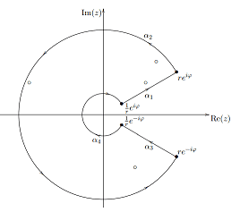 Observe that
$$
f(z),dx:={(-z)}^{lambda -1}R(z)=expleft((lambda -1)log(-z)proper)R(z)
$$
is holomorphic for ##zin mathbb{C}backslash mathbb{R}^+## if we selected the principle department of the complicated logarithm. We outline a closed curve
$$
alpha=start{instances}
alpha_1(t)=te^{ivarphi }&textual content{ if } tin left[1/r,rright]
alpha_2(t)=re^{it}&textual content{ if }t inleft[varphi ,2pi -varphi right]
alpha_3(t)=-te^{-ivarphi }&textual content{ if }tin left[-r,-1/rright]
alpha_4(t)=frac{1}{r}e^{i (2pi-t)}&textual content{ if }tin left[varphi ,2pi – varphi right]
finish{instances}
$$
such that the poles are all enclosed by ##alpha## for big sufficient ##r## and sufficiently small ##varphi## and
$$
int_{alpha_1}f(z),dz+underbrace{int_{alpha_2}f(z),dz}_{stackrel{varphi to 0}{longrightarrow },0}+int_{alpha_3}f(z),dz+underbrace{int_{alpha_4}f(z),dz}_{stackrel{varphi to 0}{longrightarrow },0}=2pi i sum_{z_k}operatorname{Res}_{z_k}left(fright)
$$
We will present that
start{align*}
displaystyle{lim_{varphi to 0}}&int_{alpha_1}f(z),dz=-e^{-lambda pi i}int_{1/r}^r t^{lambda -1}R(t),dt
displaystyle{lim_{varphi to 0}}&int_{alpha_3}f(z),dz=e^{lambda pi i}int_{1/r}^r t^{lambda -1}R(t),dt
finish{align*}
and at last get
$$
2pi i sum_{z_k}operatorname{Res}_{z_k}left(fright) =lim_{r to infty}int_alpha f(t),dt=2 i sin(lambda pi) int_{-infty }^infty t^{lambda -1}R(t),dt.
$$
The sinc Perform.
The sinc perform is outlined as ##operatorname{sinc}(x)=dfrac{sin x}{x}## for ##xneq 0## and ##operatorname{sinc(0)=1}.##
start{align*}
int_0^infty dfrac{sin x}{x},dx&=dfrac{1}{2}lim_{r to infty}int_{-r}^rdfrac{e^{iz}-e^{-iz}}{2i z},dz=operatorname{Res}_0left(dfrac{e^{iz}}{4 i z}proper)=dfrac{pi}{2}
finish{align*}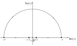
Guidelines for Residues.
We lastly embrace some basic calculation guidelines for residue calculus that we took from [7].
$$
start{array}{ll} operatorname{Res}_{z_0}(alpha f+beta g)=alphaoperatorname{Res}_{z_0}(f)+betaoperatorname{Res}_{z_0}(g) &(z_0in G , , ,alpha, beta in mathbb{C}) [16pt] operatorname{Res}_{z_1}left(dfrac{h}{f}proper)=dfrac{h(z_1)}{f'(z_1)}& operatorname{Res}_{z_1}left(dfrac{1}{f}proper)=dfrac{1}{f'(z_1)}[16pt] operatorname{Res}_{z_m}left(hdfrac{f’}{f}proper)=h(z_m)cdot m&operatorname{Res}_{z_m}left(dfrac{f’}{f}proper)=m[16pt] operatorname{Res}_{p_1}(hcdot f)=h(p_1)cdot operatorname{Res}_{p_1}(f)&operatorname{Res}_{p_1}(f)=displaystyle{lim_{z to p_1}((z-p_1)f(z))}[16pt] operatorname{Res}_{p_m}(f)=dfrac{1}{(m-1)!}displaystyle{lim_{z to p_m}dfrac{partial^{m-1} }{partial z^{m-1}}left( (z-p_m)^m f(z) proper)}&operatorname{Res}_{p_m}left(dfrac{f’}{f}proper)=-m[16pt] operatorname{Res}_{infty }(f)=operatorname{Res}_0left(-dfrac{1}{z^2}fleft(dfrac{1}{z}proper)proper)&operatorname{Res}_{p_m}left(hdfrac{f’}{f}proper)=-h(p_m)cdot m[16pt] operatorname{Res}_{z_0}(h)=0 & operatorname{Res}_0left(dfrac{1}{z}proper)=1[16pt] operatorname{Res}_1left(dfrac{z}{z^2-1}proper)=operatorname{Res}_{-1}left(dfrac{z}{z^2-1}proper)=dfrac{1}{2}&operatorname{Res}_0left(dfrac{e^z}{z^m}proper)=dfrac{1}{(m-1)!}
finish{array}
$$
Sources
[ad_2]